ARMA: one recursion for fitting and forecasting#
An ARMA(1,1) model feeds both the previous observation and the previous prediction
error into its next prediction. This is the smallest example of the ssoe
(single source of error) helper. Synthetic data let us inspect parameter recovery,
and a rolling-origin backtest checks predictions on multiple held-out windows.
Inspired by Juan Orduz’s ARMA notebook. The implementation uses PyMC parameters, named coordinates, and one shared update rule.
Prepare notebook#
import os

import arviz as az
import matplotlib.pyplot as plt
import numpy as np
import pandas as pd
import pymc as pm
import xarray as xr

from pymc_forecast import (
    HMCForecaster,
    Horizon,
    backtest,
    evaluate_forecast,
    results_to_dataframe,
    ssoe,
)

SMOKE = os.getenv("PYMC_FORECAST_SMOKE_TEST") == "1"
SEED = 2026
rng = np.random.default_rng(SEED)
DRAWS, TUNE, CHAINS = (25, 25, 1) if SMOKE else (600, 800, 2)
N_PRED = 50 if SMOKE else 800
HDI_PROB = 0.94

az.style.use("arviz-darkgrid")
if "stats.ci_kind" in az.rcParams:  # ArviZ 1.x; ArviZ 0.x intervals are always HDI
    az.rcParams["stats.ci_kind"] = "hdi"
az.rcParams["stats.ci_prob"] = HDI_PROB
plt.rcParams["figure.figsize"] = [10, 6]
plt.rcParams["figure.dpi"] = 100
plt.rcParams["figure.facecolor"] = "white"

%config InlineBackend.figure_format = "retina"
print(
    "Execution mode:", "CI smoke check; do not interpret fit quality" if SMOKE else "full example"
)
Execution mode: full example
Simulate a known process#
phi_true, theta_true, sigma_true = 0.65, 0.25, 0.4
n_train, horizon = 140, 24
errors = rng.normal(0, sigma_true, n_train + horizon)
values = np.zeros(n_train + horizon)
previous_y = previous_error = 0.0
for i, error in enumerate(errors):
    values[i] = phi_true * previous_y + theta_true * previous_error + error
    previous_y, previous_error = values[i], error
series = xr.DataArray(
    values, dims="time", coords={"time": pd.date_range("2024-01-01", periods=len(values), freq="D")}
)
train = series.isel(time=slice(n_train))
truth = series.isel(time=slice(n_train, None)).rename(time="time_future")
Define the recursion#
\(\mu_t=\phi y_{t-1}+\theta\epsilon_{t-1}\) and \(y_t=\mu_t+\epsilon_t\).
During training, the filter computes errors from observations. During forecasting,
eps_future is absent from the posterior and is sampled anew; simulated observations
and errors update the same state. Stationarity and invertibility are enforced here
by bounding the two coefficients. Initial observation and error are fixed at zero,
matching this simulation; real data may call for an inferred initial state.
ssoe registers only future errors. We explicitly register the likelihood and
predictions, so future observation noise is included exactly once.
def arma_model(covariates, data=None):
    h = Horizon.from_data(covariates, data)
    phi = pm.Uniform("phi", -0.95, 0.95)
    theta = pm.Uniform("theta", -0.95, 0.95)
    sigma = pm.HalfNormal("sigma", 1.0)

    def mean(state, x, phi, theta):
        previous_y, previous_error = state
        return phi * previous_y + theta * previous_error

    def update(state, y, error, x, phi, theta):
        return y, error

    r = ssoe(
        h,
        "eps",
        None,
        (0.0, 0.0),
        mean,
        update,
        pm.Normal.dist(0, sigma),
        params=(phi, theta),
    )
    pm.Normal("obs", r.mu, sigma, observed=h.data.values, dims="time")
    pm.Deterministic("mu", r.mu, dims="time")
    if h.future:
        pm.Deterministic("mu_future", r.mu_future, dims="time_future")
        pm.Deterministic("forecast", r.y_future, dims="time_future")
Fit and inspect parameter recovery#
fc = HMCForecaster(
    arma_model,
    train,
    draws=DRAWS,
    tune=TUNE,
    chains=CHAINS,
    random_seed=SEED,
    progressbar=False,
    sample_kwargs={"target_accept": 0.9},
)
summary = az.summary(fc.idata, var_names=["phi", "theta", "sigma"])
summary["simulation_truth"] = [phi_true, theta_true, sigma_true]
summary
Initializing NUTS using jitter+adapt_diag...
Multiprocess sampling (2 chains in 2 jobs)
NUTS: [phi, theta, sigma]
Sampling 2 chains for 800 tune and 600 draw iterations (1_600 + 1_200 draws total) took 1 seconds.
We recommend running at least 4 chains for robust computation of convergence diagnostics
| mean | sd | hdi94_lb | hdi94_ub | ess_bulk | ess_tail | r_hat | mcse_mean | mcse_sd | simulation_truth | |
|---|---|---|---|---|---|---|---|---|---|---|
| phi | 0.689 | 0.075 | 0.55 | 0.82 | 726 | 631 | 1.00 | 0.0028 | 0.0023 | 0.65 |
| theta | 0.298 | 0.092 | 0.13 | 0.47 | 899 | 807 | 1.00 | 0.0031 | 0.0028 | 0.25 |
| sigma | 0.429 | 0.026 | 0.38 | 0.48 | 960 | 916 | 1.00 | 0.00084 | 0.00072 | 0.4 |
Forecast with one fixed set of posterior draws#
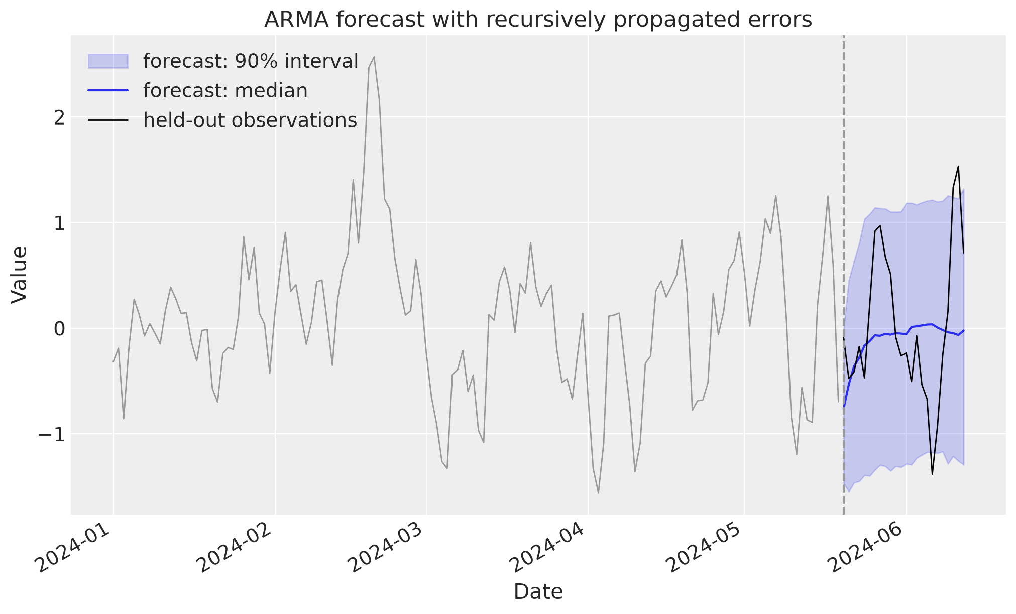
mu_future excludes each step’s current observation error. It still varies with
errors simulated at earlier future steps. This is the conditional one-step mean,
not an unconditional multi-step expectation that integrates all future errors.
posterior = fc.draw_posterior(N_PRED, random_seed=SEED + 1)
pred = fc.forecast(horizon=horizon, posterior=posterior, random_seed=SEED + 2).predictions
np.testing.assert_allclose(pred.forecast - pred.mu_future, pred.eps_future)
assert pred.forecast.dims == ("chain", "draw", "time_future")
pd.Series(evaluate_forecast(pred.forecast, truth))
Sampling: [eps_future]
mae         0.569283
rmse        0.724103
crps        0.409667
coverage    0.875000
dtype: float64
def plot_forecast(ax, samples, truth, label="forecast", color="C0"):
    time = samples.time_future.values
    q = samples.quantile([0.05, 0.5, 0.95], dim=("chain", "draw"))
    ax.fill_between(
        time,
        q.sel(quantile=0.05),
        q.sel(quantile=0.95),
        alpha=0.2,
        color=color,
        label=f"{label}: 90% interval",
    )
    ax.plot(time, q.sel(quantile=0.5), color=color, label=f"{label}: median")
    ax.plot(time, truth.values, color="black", lw=1, label="held-out observations")
    ax.set(xlabel="Date", ylabel="Value")
    ax.legend(loc="upper left")
fig, ax = plt.subplots()
plot_forecast(ax, pred.forecast, truth)
ax.plot(train.time, train, color="0.6", lw=1)
ax.axvline(truth.time_future.values[0], color="0.6", ls="--")
ax.set_title("ARMA forecast with recursively propagated errors")
fig.autofmt_xdate()
plt.show()
Expanding-window backtest#
Every fold refits on its own history; the errors of the held-out observations never enter the recursion. Scores include observation noise and are computed on the original scale. Two small folds keep this example inexpensive.
results = backtest(
    series,
    None,
    arma_model,
    forecaster_cls=HMCForecaster,
    min_train_window=116,
    test_window=24,
    stride=24,
    num_samples=N_PRED,
    forecaster_options={
        "draws": DRAWS,
        "tune": TUNE,
        "chains": CHAINS,
        "progressbar": False,
        "sample_kwargs": {"target_accept": 0.9},
    },
    keep_predictions=True,
    random_seed=SEED + 3,
)
results_to_dataframe(results)
Initializing NUTS using jitter+adapt_diag...
Multiprocess sampling (2 chains in 2 jobs)
NUTS: [phi, theta, sigma]
Sampling 2 chains for 800 tune and 600 draw iterations (1_600 + 1_200 draws total) took 1 seconds.
We recommend running at least 4 chains for robust computation of convergence diagnostics
Sampling: [eps_future]
Initializing NUTS using jitter+adapt_diag...
Multiprocess sampling (2 chains in 2 jobs)
NUTS: [phi, theta, sigma]
Sampling 2 chains for 800 tune and 600 draw iterations (1_600 + 1_200 draws total) took 1 seconds.
We recommend running at least 4 chains for robust computation of convergence diagnostics
Sampling: [eps_future]
| t0 | t1 | t2 | num_samples | train_walltime | test_walltime | mae | rmse | crps | coverage | |
|---|---|---|---|---|---|---|---|---|---|---|
| 0 | 0 | 116 | 140 | 800 | 1.642119 | 0.108752 | 0.643048 | 0.728495 | 0.425031 | 0.958333 |
| 1 | 0 | 140 | 164 | 800 | 1.400372 | 0.114609 | 0.553600 | 0.712774 | 0.403901 | 0.833333 |
What to inspect#
Check coefficient recovery and NUTS diagnostics before interpreting the forecasts. Compare coverage across folds as well as CRPS; a single test segment is noisy. The package tests additionally compare predictive variances against the analytical ARMA impulse-response formula, which catches implementations that drop future errors.