Univariate forecasting with `pymc_forecast`#

This notebook ports the upstream NumPyro univariate forecasting example to the PyMC API. We forecast weekly BART ridership with a random-walk local level, annual Fourier seasonality, and a Student-T likelihood, fit with variational inference and evaluated with the continuous ranked probability score (CRPS).

The data is derived from the complete hourly BART origin-destination panel used by the upstream example. All predictive results use arviz.InferenceData, and all time handling uses labeled xarray coordinates.

Prepare notebook#

import logging
import os
from functools import partial

import arviz as az
import matplotlib.pyplot as plt
import numpy as np
import pymc as pm
import pytensor.tensor as pt
import xarray as xr

from pymc_forecast import (
    Forecaster,
    ForecastingModel,
    Horizon,
    backtest,
    build_model,
    eval_coverage,
    eval_crps,
    evaluate_forecast,
    fourier_features,
    predict,
    results_to_dataframe,
    time_series,
)
from pymc_forecast.data import FUTURE_DIM, TIME_DIM
from pymc_forecast.datasets import load_bart_weekly

az.style.use("arviz-darkgrid")
plt.rcParams["figure.figsize"] = [10, 6]
plt.rcParams["figure.dpi"] = 100
plt.rcParams["figure.facecolor"] = "white"

logging.getLogger("pymc").setLevel(logging.ERROR)
logging.getLogger("pytensor").setLevel(logging.ERROR)

SEED = 42

# CI executes every example notebook end-to-end with reduced settings.
SMOKE_TEST = os.environ.get("PYMC_FORECAST_SMOKE_TEST", "0") == "1"
NUM_STEPS = 300 if SMOKE_TEST else 20_000
NUM_SAMPLES = 50 if SMOKE_TEST else 1_000
BACKTEST_SAMPLES = 50 if SMOKE_TEST else 500

Read data#

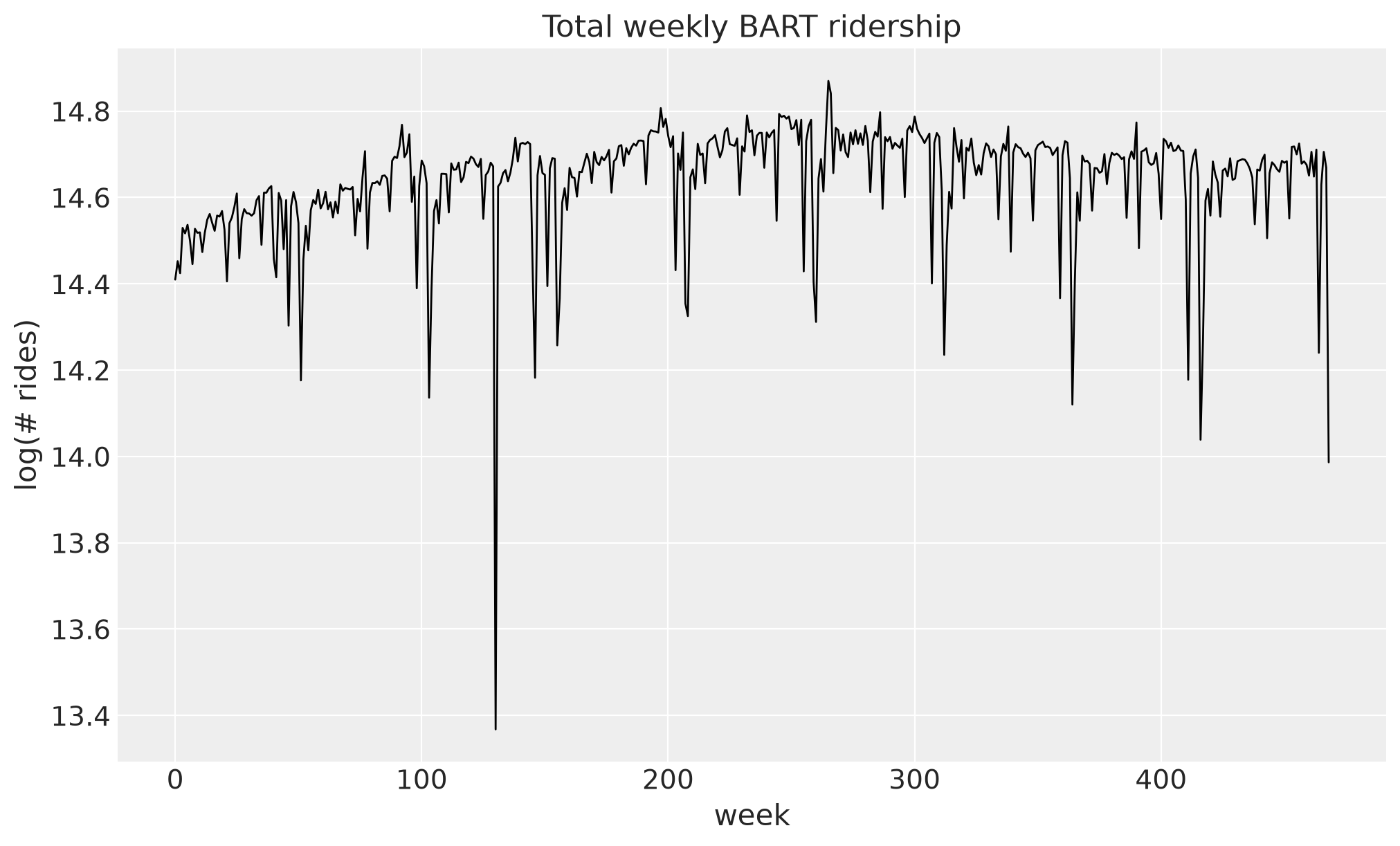
We use the same data as the upstream notebook: total weekly BART ridership. The package downloads and verifies the complete hourly origin-destination dataset, then sums over station pairs and non-overlapping weeks before applying a log transform.

y = load_bart_weekly()
duration = y.sizes[TIME_DIM]
print("weekly observations:", duration)

fig, ax = plt.subplots()
ax.plot(y[TIME_DIM].values, y.values, color="black", lw=1)
ax.set(title="Total weekly BART ridership", xlabel="week", ylabel="log(# rides)")
plt.show()

weekly observations: 469

../_images/3baa4bfe3a02fcc46f105c908d1dd94135b90cdf55a67509ff448eedbe3770ef.png

Train-test split#

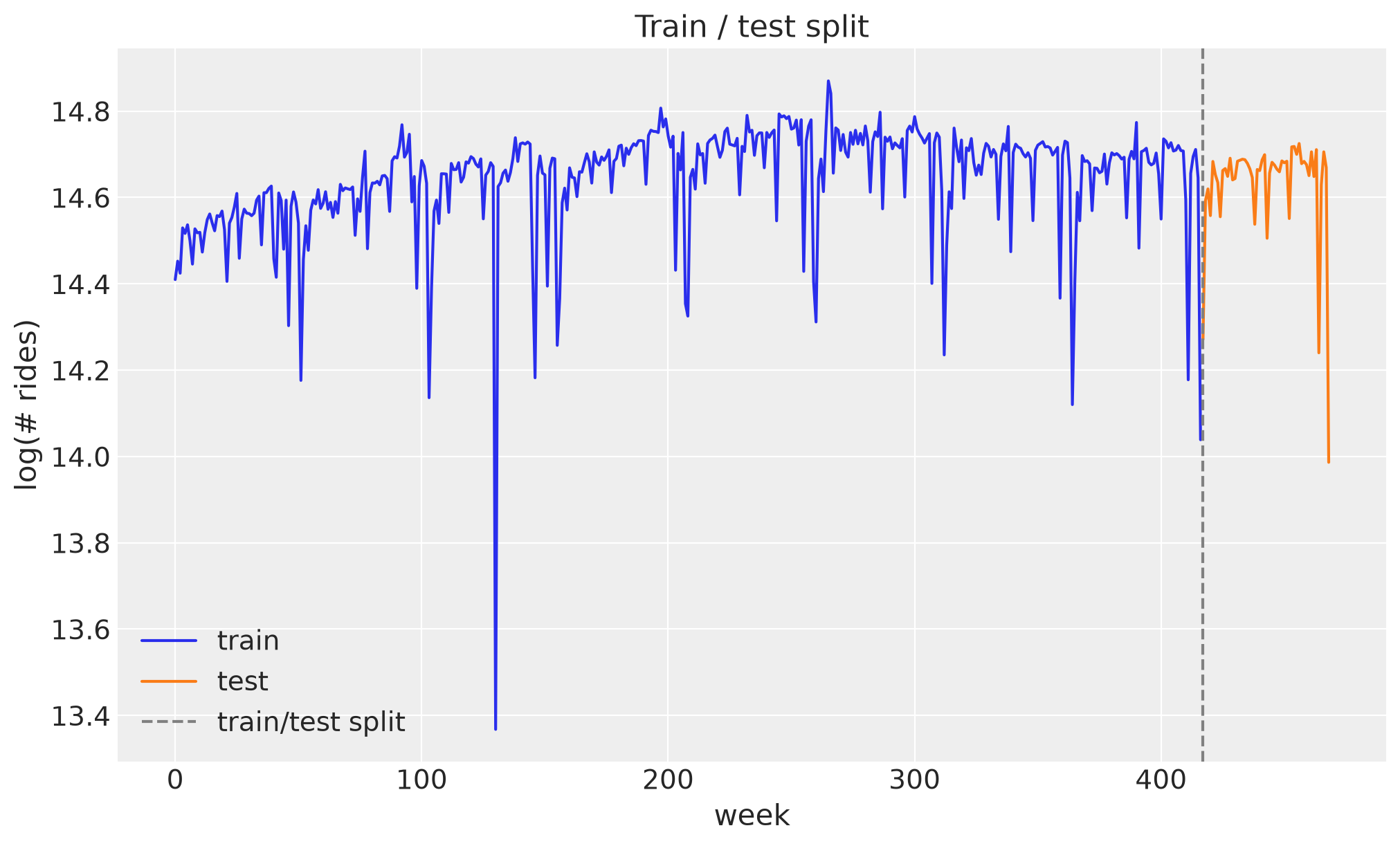
Hold out the final 52 weeks, matching the one-year forecasting horizon in the upstream example. The integer week coordinates are preserved in the predictive groups.

TEST_WINDOW = 52
T1 = duration - TEST_WINDOW

y_train = y.isel({TIME_DIM: slice(None, T1)})
y_test = y.isel({TIME_DIM: slice(T1, None)})
print("train:", y_train.sizes[TIME_DIM], "test:", y_test.sizes[TIME_DIM])

fig, ax = plt.subplots()
ax.plot(y_train[TIME_DIM].values, y_train.values, color="C0", label="train")
ax.plot(y_test[TIME_DIM].values, y_test.values, color="C1", label="test")
ax.axvline(y_test[TIME_DIM].values[0], color="gray", ls="--", label="train/test split")
ax.legend(loc="lower left")
ax.set(title="Train / test split", xlabel="week", ylabel="log(# rides)")
plt.show()

train: 417 test: 52

../_images/34da64f13399fea569b25b7d6be326367a0ad8c417a3e6fdb539e35287a94bc2.png

Seasonal features#

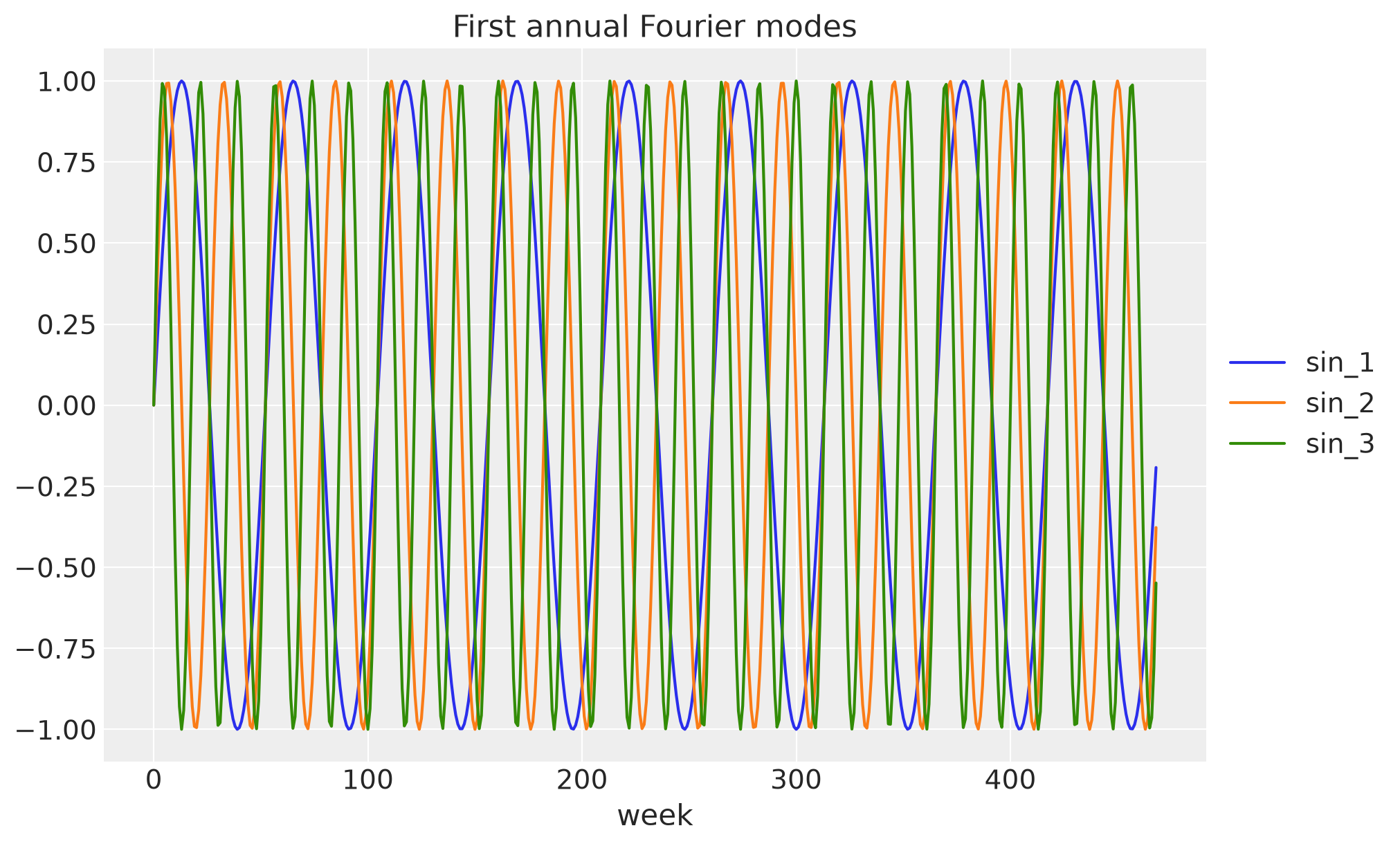
The BART series is weekly, so the seasonal design uses a 365.25 / 7 week period and 26 Fourier harmonics, matching the upstream example. Feature and observation coordinates remain aligned by week.

NUM_TERMS = 26
covariates = fourier_features(duration, period=365.25 / 7, num_terms=NUM_TERMS)
covariates = covariates.rename({"fourier": "covariate"})
covariates_train = covariates.isel({TIME_DIM: slice(None, T1)})
print("covariates:", covariates.sizes)

fig, ax = plt.subplots()
for name in covariates["covariate"].values[:3]:
    ax.plot(covariates[TIME_DIM].values, covariates.sel(covariate=name).values, label=name)
ax.legend(loc="center left", bbox_to_anchor=(1, 0.5))
ax.set(title="First annual Fourier modes", xlabel="week")
plt.show()

covariates: Frozen({'time': 469, 'covariate': 52})

../_images/e171ac13f80c992eff4dc5591f88740833585a8d8d57e01e10923395203c0392.png

Model specification#

The mean has three pieces: a global intercept, a random-walk local level, and a linear regression on Fourier features. The forecast horizon is represented by separate *_future variables through time_series, so fitting and forecasting use one model body. The random walk is non-centered for stable PyMC variational inference while retaining the upstream model’s priors.

class LocalLevelSeasonal(ForecastingModel):
    """Local level + Fourier regression with Student-T observations."""

    def model(self, h: Horizon, covariates: xr.DataArray) -> None:
        bias = pm.Normal("bias", 0.0, 10.0)
        weight = pm.Normal("weight", 0.0, 0.1, dims="covariate")
        drift_scale = pm.LogNormal("drift_scale", -20.0, 5.0, initval=0.01)
        nu = pm.Gamma("nu", alpha=10.0, beta=2.0)
        sigma = pm.LogNormal("sigma", -5.0, 5.0, initval=0.05)

        drift_raw = self.time_series(
            "drift_raw",
            lambda name, dims: pm.Normal(name, 0.0, 1.0, dims=dims),
        )
        level = pt.cumsum(drift_raw * drift_scale)
        regression = pt.dot(covariates.values, weight)
        prediction = bias + level + regression

        self.predict(
            lambda name, mu, dims, observed: pm.StudentT(
                name,
                nu=nu,
                mu=mu,
                sigma=sigma,
                dims=dims,
                observed=observed,
            ),
            prediction,
        )


model = LocalLevelSeasonal()
train_model = build_model(model, y_train, covariates_train)
train_model

\[\begin{split} \begin{array}{rcl} \text{bias} &\sim & \operatorname{Normal}(0,~10)\\\text{weight} &\sim & \operatorname{Normal}(0,~0.1)\\\text{drift\_scale} &\sim & \operatorname{LogNormal}(-20,~5)\\\text{nu} &\sim & \operatorname{Gamma}(10,~\text{<constant>})\\\text{sigma} &\sim & \operatorname{LogNormal}(-5,~5)\\\text{drift\_raw} &\sim & \operatorname{Normal}(0,~1)\\\text{obs} &\sim & \operatorname{StudentT}(\text{nu},~f(\text{bias},~\text{weight},~\text{drift\_raw},~\text{drift\_scale}),~\text{sigma}) \end{array} \end{split}\]

Plot helper#

def attach_constant_data(idata, *, name: str, values: np.ndarray, dim: str) -> None:
    """Add an ArviZ constant-data group used by plot_lm."""
    idata["constant_data"] = xr.Dataset(
        {name: (dim, np.asarray(values, dtype=float))},
        coords={dim: idata["observed_data"][dim].values},
    )


def lm_idata_from_forecast(
    samples: xr.DataArray,
    truth: xr.DataArray,
    *,
    x_name: str,
    x_values: np.ndarray,
):
    """Represent held-out forecasts as an ArviZ posterior predictive container."""
    return az.from_dict(
        {
            "posterior_predictive": {"obs": samples.values},
            "observed_data": {"obs": truth.values},
            "constant_data": {x_name: np.asarray(x_values, dtype=float)},
        },
        coords={TIME_DIM: truth[FUTURE_DIM].values},
        dims={"obs": [TIME_DIM], x_name: [TIME_DIM]},
    )

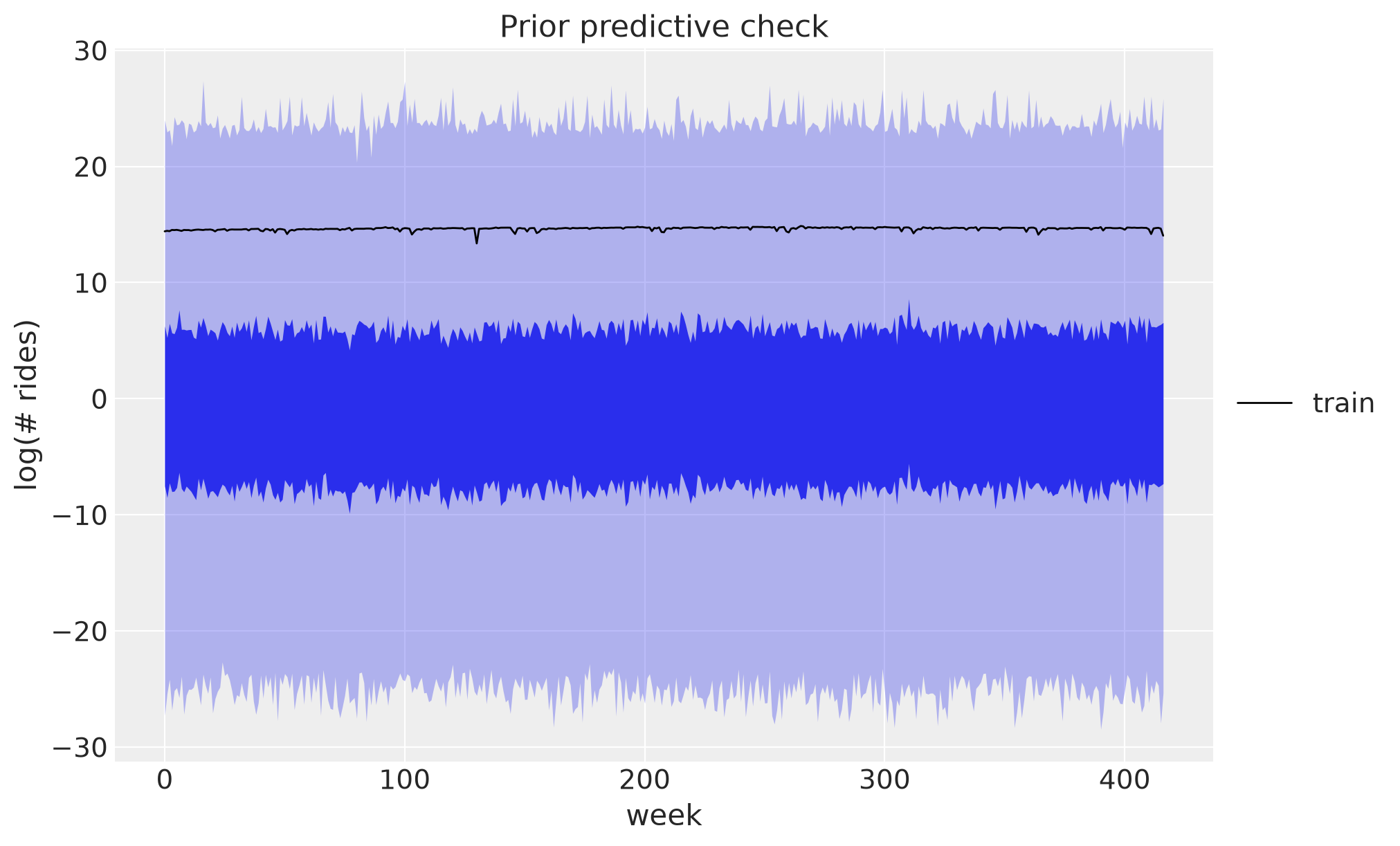
Prior predictive checks#

prior_model = build_model(model, y_train, covariates_train)
prior_idata = pm.sample_prior_predictive(
    draws=NUM_SAMPLES,
    model=prior_model,
    var_names=["obs"],
    random_seed=SEED,
)
attach_constant_data(
    prior_idata,
    name="week",
    values=y_train[TIME_DIM].values,
    dim=TIME_DIM,
)

prior_pc = az.plot_lm(
    prior_idata,
    y="obs",
    x="week",
    group="prior_predictive",
    ci_kind="hdi",
    ci_prob=(0.5, 0.94),
    smooth=False,
    visuals={
        "ci_band": {"color": "C0"},
        "observed_scatter": False,
        "pe_line": False,
    },
    figure_kwargs={"figsize": (10, 6)},
)
ax = prior_pc.viz["figure"].item().axes[0]
ax.plot(y_train[TIME_DIM].values, y_train.values, color="black", lw=1, label="train")
ax.legend(loc="center left", bbox_to_anchor=(1, 0.5))
ax.set(title="Prior predictive check", xlabel="week", ylabel="log(# rides)")
plt.show()

../_images/b643d7e9d11ec66c4ecd981f90a10d238fadf71432f37d8afb529d64f3d1dea0.png

Inference with ADVI#

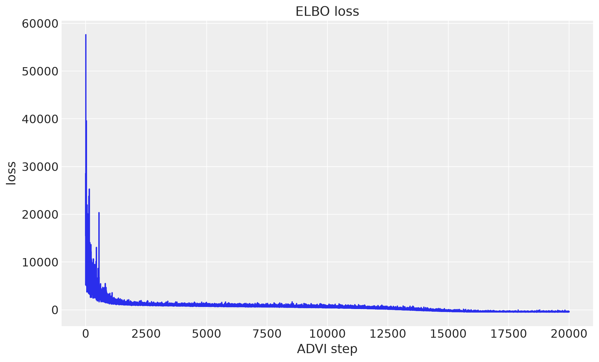
Forecaster fits the model with PyMC variational inference. The non-centered random walk keeps the high-dimensional weekly latent trajectory tractable for ADVI.

forecaster = Forecaster(
    model,
    y_train,
    covariates_train,
    optimizer=0.005,
    num_steps=NUM_STEPS,
    random_seed=SEED,
    progressbar=False,
)

fig, ax = plt.subplots()
ax.plot(forecaster.losses)
ax.set(title="ELBO loss", xlabel="ADVI step", ylabel="loss")
plt.show()

Posterior predictive check and forecast#

train_pp_idata = forecaster.predict_in_sample(
    num_samples=NUM_SAMPLES,
    random_seed=SEED,
    progressbar=False,
)
forecast_idata = forecaster.forecast(
    covariates,
    num_samples=NUM_SAMPLES,
    random_seed=SEED,
    progressbar=False,
)
attach_constant_data(
    train_pp_idata,
    name="week",
    values=y_train[TIME_DIM].values,
    dim=TIME_DIM,
)

train_pp = train_pp_idata["posterior_predictive"]["obs"]
forecast = forecast_idata["predictions"]["forecast"]
forecast_lm_idata = lm_idata_from_forecast(
    forecast,
    y_test.rename({TIME_DIM: FUTURE_DIM}),
    x_name="week",
    x_values=y_test[TIME_DIM].values,
)

metrics = {
    "crps": eval_crps,
    "coverage_50": partial(eval_coverage, alpha=0.5),
    "coverage_94": partial(eval_coverage, alpha=0.94),
}
train_scores = evaluate_forecast(train_pp, y_train, metrics=metrics)
test_scores = evaluate_forecast(forecast, y_test.rename({TIME_DIM: FUTURE_DIM}), metrics=metrics)
print("train:", train_scores)
print("test: ", test_scores)

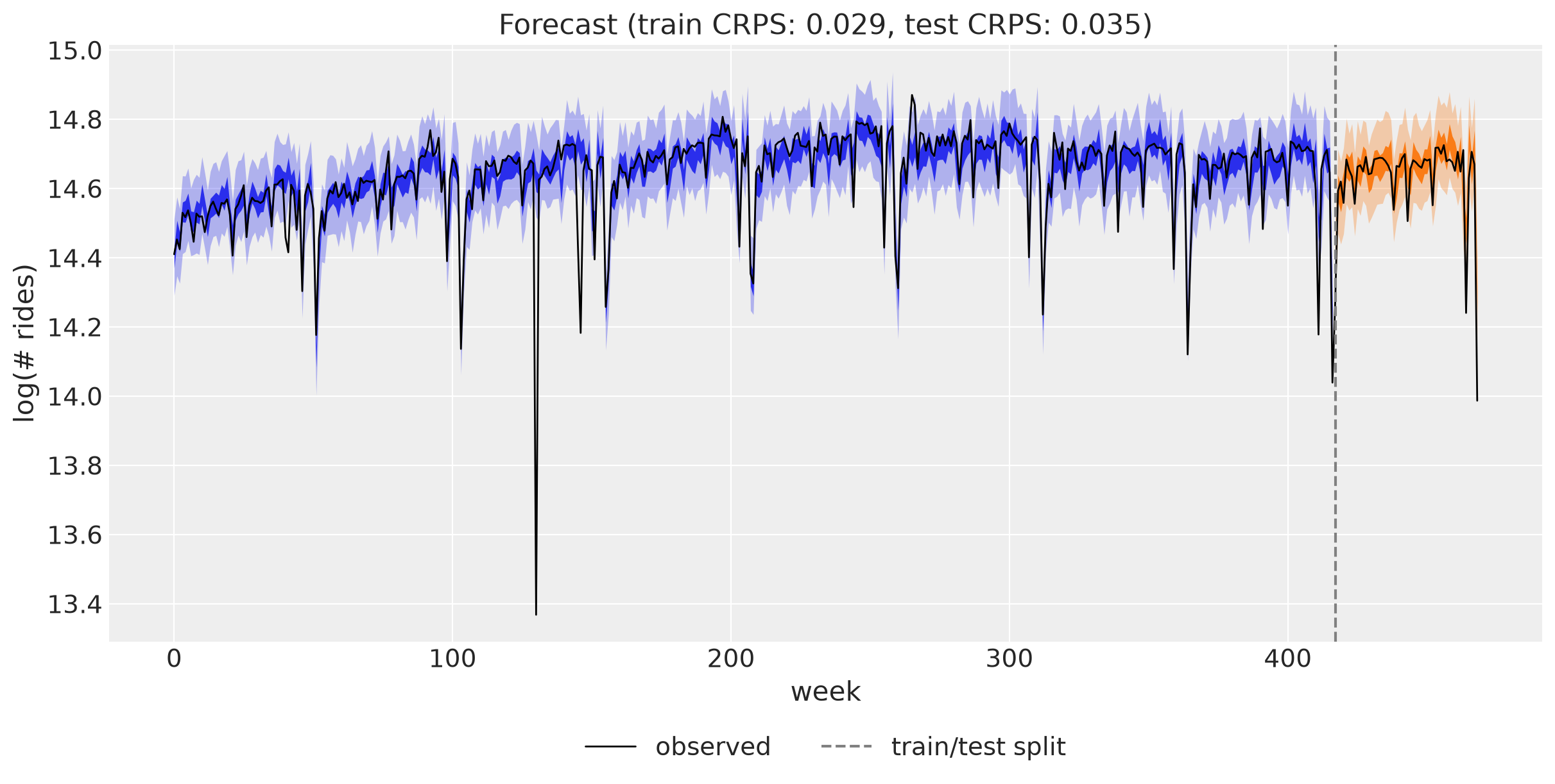
train: {'crps': 0.028555026889263202, 'coverage_50': 0.6378896882494005, 'coverage_94': 0.9640287769784173}
test:  {'crps': 0.03481793016505593, 'coverage_50': 0.6346153846153846, 'coverage_94': 0.9038461538461539}

Forecast visualization#

forecast_title = (
    f"Forecast (train CRPS: {train_scores['crps']:.3f}, test CRPS: {test_scores['crps']:.3f})"
)

pc = az.plot_lm(
    train_pp_idata,
    y="obs",
    x="week",
    ci_kind="hdi",
    ci_prob=(0.5, 0.94),
    smooth=False,
    visuals={"ci_band": {"color": "C0"}, "observed_scatter": False, "pe_line": False},
    figure_kwargs={"figsize": (12, 6)},
)
az.plot_lm(
    forecast_lm_idata,
    y="obs",
    x="week",
    plot_collection=pc,
    ci_kind="hdi",
    ci_prob=(0.5, 0.94),
    smooth=False,
    visuals={"ci_band": {"color": "C1"}, "observed_scatter": False, "pe_line": False},
)
ax = pc.viz["figure"].item().axes[0]
ax.plot(y[TIME_DIM].values, y.values, color="black", lw=1, label="observed")
ax.axvline(T1, color="gray", ls="--", label="train/test split")
ax.legend(loc="upper center", bbox_to_anchor=(0.5, -0.12), ncol=3)
ax.set(title=forecast_title, xlabel="week", ylabel="log(# rides)")
plt.show()

../_images/725077936abe0489a831afe7ad3e0124a677163f0a09ff7ec5145a17556be937.png

Rolling-origin backtesting#

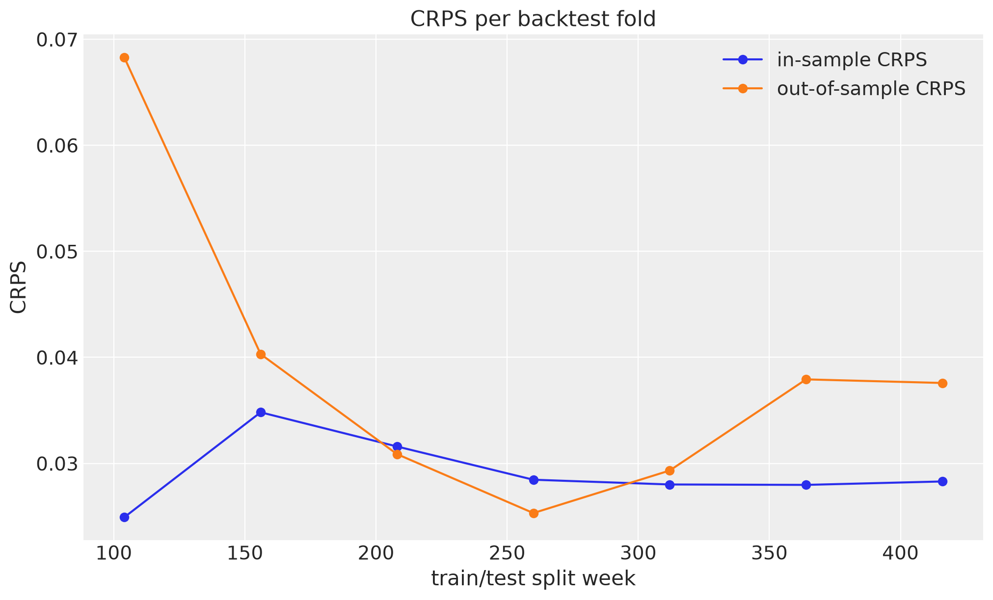
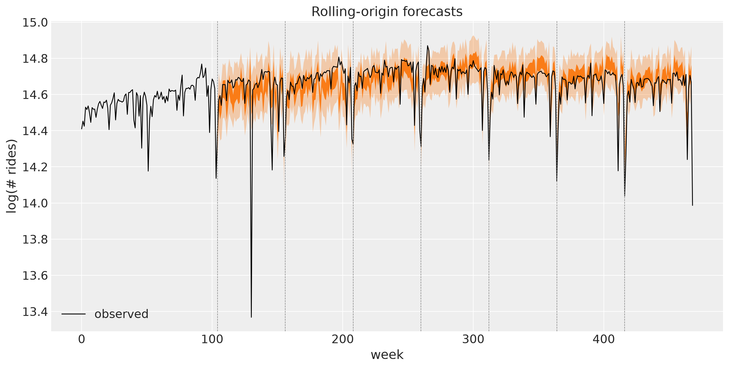
The supported PyMC API refits expanding windows one fold at a time. Each fold forecasts one year, advances one year, and keeps predictions labeled by their real week coordinates. The upstream JAX-only vectorized backtest is intentionally omitted.

backtest_model = LocalLevelSeasonal()
results = backtest(
    y,
    covariates,
    backtest_model,
    metrics=metrics,
    test_window=52,
    stride=52,
    min_train_window=104,
    min_test_window=52,
    num_samples=BACKTEST_SAMPLES,
    eval_train=True,
    keep_predictions=True,
    forecaster_options={"optimizer": 0.005, "num_steps": NUM_STEPS},
    random_seed=SEED,
)
summary = results_to_dataframe(results)
summary

	t1	t2	num_samples	train_walltime	test_walltime	crps	coverage_50	coverage_94	train_crps	train_coverage_50	train_coverage_94
0	104	156	500	72.068933	3.894191	0.068290	0.442308	0.942308	0.024918	0.855769	0.990385
1	156	208	500	57.775307	2.593398	0.040307	0.519231	0.923077	0.034820	0.743590	0.980769
2	208	260	500	43.358285	0.944961	0.030875	0.557692	0.980769	0.031596	0.716346	0.971154
3	260	312	500	75.345317	2.871415	0.025316	0.673077	0.980769	0.028461	0.726923	0.973077
4	312	364	500	50.631031	1.919438	0.029328	0.557692	0.980769	0.028013	0.692308	0.967949
5	364	416	500	13.027945	2.657666	0.037924	0.423077	0.903846	0.027974	0.689560	0.969780
6	416	468	500	29.529265	0.547134	0.037585	0.461538	0.903846	0.028298	0.653846	0.966346

fig, ax = plt.subplots()
ax.plot(summary["t1"], summary["train_crps"], "o-", color="C0", label="in-sample CRPS")
ax.plot(summary["t1"], summary["crps"], "o-", color="C1", label="out-of-sample CRPS")
ax.legend()
ax.set(xlabel="train/test split week", ylabel="CRPS", title="CRPS per backtest fold")
plt.show()

../_images/06ce6cf421009f4d9bd5cca5ca4e60fd4112fc5a22b175c6958ccf52cdbbcdee.png

pc = None
for result in results:
    if result.prediction is None:
        continue
    truth = y.isel({TIME_DIM: slice(result.t1, result.t2)}).rename({TIME_DIM: FUTURE_DIM})
    fold_idata = lm_idata_from_forecast(
        result.prediction,
        truth,
        x_name="week",
        x_values=np.arange(result.t1, result.t2),
    )
    if pc is None:
        pc = az.plot_lm(
            fold_idata,
            y="obs",
            x="week",
            ci_kind="hdi",
            ci_prob=(0.5, 0.94),
            smooth=False,
            visuals={"ci_band": {"color": "C1"}, "observed_scatter": False, "pe_line": False},
            figure_kwargs={"figsize": (12, 6)},
        )
    else:
        az.plot_lm(
            fold_idata,
            y="obs",
            x="week",
            plot_collection=pc,
            ci_kind="hdi",
            ci_prob=(0.5, 0.94),
            smooth=False,
            visuals={"ci_band": {"color": "C1"}, "observed_scatter": False, "pe_line": False},
        )

if pc is None:
    msg = "no folds were plotted"
    raise ValueError(msg)
ax = pc.viz["figure"].item().axes[0]
ax.plot(y[TIME_DIM].values, y.values, color="black", lw=1, label="observed")
for result in results:
    ax.axvline(result.t1, color="gray", ls="--", lw=0.6)
ax.legend(loc="lower left")
ax.set(title="Rolling-origin forecasts", xlabel="week", ylabel="log(# rides)")
plt.show()

../_images/d2ebf6aaa326c936400a30cbc070f2ac5c1c8f12718de374f1962dcb05435586.png

Functional API#

def local_level_seasonal(h: Horizon, covariates: xr.DataArray) -> None:
    """Functional twin of ``LocalLevelSeasonal.model``."""
    bias = pm.Normal("bias", 0.0, 10.0)
    weight = pm.Normal("weight", 0.0, 0.1, dims="covariate")
    drift_scale = pm.LogNormal("drift_scale", -20.0, 5.0, initval=0.01)
    nu = pm.Gamma("nu", alpha=10.0, beta=2.0)
    sigma = pm.LogNormal("sigma", -5.0, 5.0, initval=0.05)

    drift_raw = time_series(
        h,
        "drift_raw",
        lambda name, dims: pm.Normal(name, 0.0, 1.0, dims=dims),
    )
    level = pt.cumsum(drift_raw * drift_scale)
    regression = pt.dot(covariates.values, weight)

    predict(
        h,
        lambda name, mu, dims, observed: pm.StudentT(
            name,
            nu=nu,
            mu=mu,
            sigma=sigma,
            dims=dims,
            observed=observed,
        ),
        bias + level + regression,
    )


oop_names = list(build_model(LocalLevelSeasonal(), y_train, covariates_train).named_vars)
functional_names = list(build_model(local_level_seasonal, y_train, covariates_train).named_vars)
print("same named variables:", oop_names == functional_names)
print(functional_names)

same named variables: True
['bias', 'weight', 'drift_scale', 'nu', 'sigma', 'drift_raw', 'obs']

References#

Upstream NumPyro notebook: https://github.com/juanitorduz/numpyro_forecast/blob/main/docs/examples/forecasting_univariate.ipynb
Pyro BART dataset mirror: https://github.com/pyro-ppl/datasets/tree/master/bart
Juan Orduz, Univariate time series forecasting with NumPyro: https://juanitorduz.github.io/numpyro_forecasting-univariate/

Univariate forecasting with pymc_forecast#