Demand forecasting with a censored likelihood#

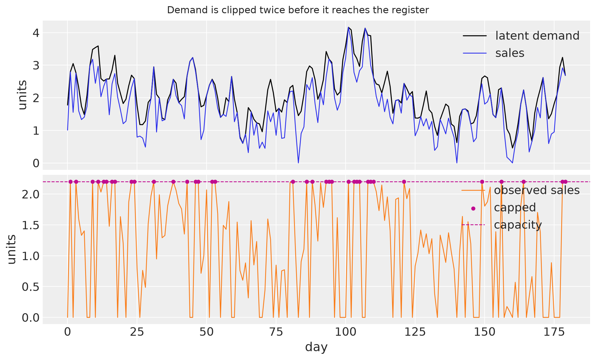
Recorded sales understate demand in two ways. A stockout writes a genuine demand day as zero. A shelf that cannot hold any more stops the register at a capacity cap, so the recorded number is a lower bound. A model trained on that series forecasts sales. Replenishment needs a forecast of demand.

This notebook simulates an AR(2) with weekly seasonality, censors it, and fits one ForecastingModel whose likelihood knows the difference: a normal density below the cap, survival mass at the cap, and no contribution from stockout days. The same recursion filters the training history and simulates the horizon. It is a port of the numpyro-forecast censored-demand example, which itself ports Demand Forecasting with Censored Likelihood.

The sibling examples treat availability differently. Intermittent demand separates occurrence from size. Retail stockouts scales the mean by a floored availability factor. Here the censoring point is known, so the likelihood models the mechanism instead of its average effect.

Prepare notebook#

import os
from functools import partial

import arviz as az
import jax
import jax.numpy as jnp
import matplotlib.pyplot as plt
import numpy as np
import pandas as pd
import pymc as pm
import pytensor.tensor as pt
import xarray as xr
from IPython.display import display
from jax import random

from pymc_forecast import (
    ForecastingModel,
    HMCForecaster,
    eval_coverage,
    eval_crps,
    eval_mae,
    eval_rmse,
    evaluate_forecast,
    fourier_features,
    ssoe,
)

SMOKE = os.getenv("PYMC_FORECAST_SMOKE_TEST") == "1"
SEED = 42
DRAWS, TUNE, CHAINS = (25, 25, 1) if SMOKE else (1000, 1000, 4)
N_PERIODS = 48 if SMOKE else 180
HORIZON = 12 if SMOKE else 30
CAPACITY = np.float32(2.2)
HDI_PROB = 0.94

az.style.use("arviz-darkgrid")
if "stats.ci_kind" in az.rcParams:  # ArviZ 1.x; ArviZ 0.x intervals are always HDI
    az.rcParams["stats.ci_kind"] = "hdi"
az.rcParams["stats.ci_prob"] = HDI_PROB
plt.rcParams["figure.figsize"] = [10, 6]
plt.rcParams["figure.dpi"] = 100
plt.rcParams["figure.facecolor"] = "white"

%config InlineBackend.figure_format = "retina"
print(
    "Execution mode:",
    "CI smoke check; do not interpret fit quality" if SMOKE else "full example",
)
print("jax", jax.__version__)

Execution mode: full example
jax 0.11.2

Simulate demand, sales, and the register#

Latent demand is an AR(2) plus a weekly sinusoid, clipped at zero. Sales are demand minus friction, never above demand and never negative. Observed sales are zero when the product is off the shelf and capped at 2.2 otherwise.

\[ d_t = \max(0, \phi_1 d_{t-1} + \phi_2 d_{t-2} + \gamma \sin(2\pi t / 7) + \alpha + \varepsilon^d_t) \]

\[ s_t = \max(0, \min(d_t + \varepsilon^s_t - \delta, d_t)), \qquad y_t = \min(a_t s_t, 2.2) \]

The censoring indicator is \(c_t = 1\{y_t = 2.2\}\). Equality is safe here because the simulation’s minimum returns the cap bit-exactly. The seed and the split match the upstream notebook, so the 180-day series has the same 49 stockouts and 36 capped days.

def generate_demand_sales(key, n_periods=180):
    """Simulate latent demand, uncapped sales, observed sales, and availability."""
    key_demand, key_sales, key_avail = random.split(key, 3)
    noise_demand = 0.3 * random.normal(key_demand, (n_periods,))
    noise_sales = 0.5 * random.normal(key_sales, (n_periods,))
    available = random.bernoulli(key_avail, 0.8, (n_periods,)).astype(jnp.float32)
    t_grid = jnp.arange(n_periods, dtype=jnp.float32)

    def step(carry, xs):
        previous_1, previous_2 = carry
        t, eps_demand, eps_sales = xs
        seasonal = 0.6 * jnp.sin(2 * jnp.pi * t / 7)
        demand = jnp.clip(
            0.6 * previous_1 + 0.3 * previous_2 + seasonal + 0.2 + eps_demand,
            min=0.0,
        )
        sales = jnp.clip(jnp.minimum(demand + eps_sales - 0.25, demand), min=0.0)
        return (demand, previous_1), (demand, sales)

    init = (jnp.float32(2.0), jnp.float32(2.0))
    _, (demand, sales) = jax.lax.scan(step, init, (t_grid, noise_demand, noise_sales))
    sales_obs = jnp.minimum(available * sales, CAPACITY)
    censored = (sales_obs == CAPACITY).astype(jnp.float32)
    return {
        "demand": np.asarray(demand),
        "sales": np.asarray(sales),
        "sales_obs": np.asarray(sales_obs),
        "available": np.asarray(available),
        "censored": np.asarray(censored),
    }


key = random.PRNGKey(SEED)
_, subkey = random.split(key)
full = generate_demand_sales(subkey, 180)
n_stockout = int((1 - full["available"]).sum())
n_censored = int(full["censored"].sum())
print(f"full series stockouts: {n_stockout}; capacity-censored days: {n_censored}")
assert n_stockout == 49
assert n_censored == 36

series = {name: values[:N_PERIODS] for name, values in full.items()}
n_train = N_PERIODS - HORIZON
time = np.arange(N_PERIODS)
print(
    f"window: {N_PERIODS} days, train {n_train}, horizon {HORIZON}; "
    f"train stockouts {int((1 - series['available'][:n_train]).sum())}, "
    f"train capped {int(series['censored'][:n_train].sum())}, "
    f"test peaks {int((series['demand'][n_train:] > CAPACITY).sum())}"
)
assert int((1 - series["available"][:n_train]).sum()) >= 1
assert int(series["censored"][:n_train].sum()) >= 1
assert int((series["demand"][n_train:] > CAPACITY).sum()) >= 1

full series stockouts: 49; capacity-censored days: 36
window: 180 days, train 150, horizon 30; train stockouts 36, train capped 32, test peaks 10

fig, (ax_top, ax_bot) = plt.subplots(nrows=2, sharex=True, figsize=(10, 6), layout="constrained")
ax_top.plot(time, series["demand"], color="black", lw=1.2, label="latent demand")
ax_top.plot(time, series["sales"], color="C0", lw=1, label="sales")
ax_top.legend(loc="upper right")
ax_top.set(ylabel="units")
ax_bot.plot(time, series["sales_obs"], color="C1", lw=1, label="observed sales")
capped = series["censored"] == 1
ax_bot.scatter(
    time[capped],
    series["sales_obs"][capped],
    color="C3",
    s=16,
    zorder=5,
    label="capped",
)
ax_bot.axhline(float(CAPACITY), color="C3", ls="--", lw=1, label="capacity")
ax_bot.legend(loc="upper right")
ax_bot.set(xlabel="day", ylabel="units")
fig.suptitle("Demand is clipped twice before it reaches the register")
plt.show()

../_images/230d10b52438d31ee2ba345ad55c4c595774771c7708e157c722c89b28c377cb.png

Covariates are the scenario#

The last 30 days are the test window (12 in the CI smoke check). Covariates cover the whole horizon. Column order is part of the model contract: availability, the censoring indicator, then weekly Fourier terms (sine, then cosine). Future rows are an explicit scenario: on the shelf, and not capped. The model reads those rows. It does not hard-code the padding, so a different scenario is a different covariate tensor rather than an edit to the class.

The naive baseline below is the same class with the censoring column set to zero. Stockouts stay masked. Only the cap changes, from a lower bound to a pretend exact observation of 2.2.

def build_inputs(observed, available, censored, horizon):
    """Stack availability, censoring, and Fourier terms. Future rows are the scenario."""
    n_periods = len(observed)
    n_observed = n_periods - horizon
    index = np.arange(n_periods)
    fourier = fourier_features(index, period=7.0, num_terms=2).rename(fourier="input")

    def channel(name, values):
        column = np.asarray(values, dtype=float)[:, None]
        return xr.DataArray(column, dims=("time", "input"), coords={"time": index, "input": [name]})

    availability = channel("availability", np.where(index < n_observed, available, 1.0))
    capped = channel("censored", np.where(index < n_observed, censored, 0.0))
    return xr.concat([availability, capped, fourier], dim="input")


inputs = build_inputs(series["sales_obs"], series["available"], series["censored"], HORIZON)
sales_obs = xr.DataArray(series["sales_obs"], dims="time", coords={"time": time})
train = sales_obs.isel(time=slice(n_train))
assert tuple(str(v) for v in inputs.coords["input"].values) == (
    "availability",
    "censored",
    "sin_1",
    "sin_2",
    "cos_1",
    "cos_2",
)
future = inputs.isel(time=slice(n_train, None))
assert np.all(future.sel(input="availability").values == 1.0)
assert np.all(future.sel(input="censored").values == 0.0)

One recursion, a censored likelihood#

The one-step mean is an AR(2) on filtered lags plus the Fourier term.

\[ \hat{y}_t = \alpha + \phi_1 \tilde{y}_{t-1} + \phi_2 \tilde{y}_{t-2} + f_t^\top \beta \]

A stockout zero must not enter the lag. Neither must a capped day be treated as if demand stopped at the cap. The filter passes a clean observation through, floors a capped day at the prediction, and substitutes the prediction on a stockout. The carry is then clipped at zero, and shifted:

\[ \tilde{y}_t = \max\left(0,\; a_t\big[(1-c_t) y_t + c_t \max(y_t, \hat{y}_t)\big] + (1-a_t)\hat{y}_t\right) \]

The likelihood matches NumPyro’s RightCensoredDistribution. Below the cap it is the normal density. At the cap it is the survival \(P(Y \ge y_t)\), using the recorded value as the bound rather than a second equality check against 2.2. The first two steps run on placeholder lags (the first observation, twice) and, like stockouts, contribute nothing. pm.Censored is the wrong registration here: its random draw is clipped, so in-sample predictive bands could not rise above the cap. A CustomDist keeps the normal draw and replaces only the log probability.

ssoe registers future errors and nothing else. The class registers obs, the in-sample mean mu, and, when the covariate horizon is longer than the data, a nonnegative forecast. The package reserves mu for that predictor, so the intercept is intercept. Scan cannot close over random variables, so the coefficients travel in params.

N_ORDER = 2
INPUT_LABELS = ("availability", "censored", "sin_1", "sin_2", "cos_1", "cos_2")


def filtered_lag(y, pred, available, censored):
    """Carry a demand lag through stockouts and capped days."""
    on_shelf = pt.switch(pt.eq(censored, 1), pt.maximum(y, pred), y)
    carried = pt.switch(pt.eq(available, 1), on_shelf, pred)
    return pt.maximum(carried, 0.0)


def censored_logp(value, mu, sigma, censored, valid):
    """Normal density, or survival at the recorded value, or zero if invalid."""
    normal = pm.logp(pm.Normal.dist(mu, sigma), value)
    # Reflect the Normal so its log-CDF evaluates the survival tail directly.
    survival = pm.logcdf(pm.Normal.dist(-mu, sigma), -value)
    point = pt.switch(censored, survival, normal)
    return pt.switch(valid, point, 0.0)


class CensoredAR2(ForecastingModel):
    """AR(2) on filtered lags with a right-censored normal likelihood."""

    def model(self, covariates, data=None):
        labels = tuple(str(v) for v in covariates.coords["input"].values)
        if labels != INPUT_LABELS:
            raise ValueError(f"expected inputs {INPUT_LABELS}, got {labels}")
        horizon = self.horizon
        observed = horizon.data
        pm.modelcontext(None).add_coord("fourier", list(INPUT_LABELS[2:]))
        intercept = pm.Normal("intercept", 1.0, 1.0)
        phi_1 = pm.Normal("phi_1", 0.0, 1.0)
        phi_2 = pm.Normal("phi_2", 0.0, 1.0)
        sigma = pm.HalfNormal("sigma", 1.0)
        beta = pm.Normal("beta_seasonal", 0.0, 1.0, dims="fourier")

        def mean(state, x, intercept, phi_1, phi_2, beta):
            return intercept + phi_1 * state[0] + phi_2 * state[1] + pt.dot(x[2:], beta)

        def update(state, y, _error, x, intercept, phi_1, phi_2, beta):
            lag_1, _lag_2 = state
            pred = mean(state, x, intercept, phi_1, phi_2, beta)
            return filtered_lag(y, pred, x[0], x[1]), lag_1

        y0 = float(observed.values[0])
        result = ssoe(
            horizon,
            "eps",
            None,
            (y0, y0),
            mean,
            update,
            pm.Normal.dist(0, sigma),
            xs=covariates,
            params=(intercept, phi_1, phi_2, beta),
        )
        train_x = covariates.sel(time=horizon.time)
        censored = pt.as_tensor_variable(train_x.sel(input="censored").values)
        available = pt.as_tensor_variable(train_x.sel(input="availability").values)
        valid = pt.and_(pt.arange(horizon.t_obs) >= N_ORDER, pt.eq(available, 1))

        def logp(value, mu, sigma):
            return censored_logp(value, mu, sigma, censored, valid)

        pm.CustomDist(
            "obs",
            result.mu,
            sigma,
            dist=lambda mu, sigma, size: pm.Normal.dist(mu, sigma, size=size),
            logp=logp,
            observed=np.asarray(observed.transpose("time").values, dtype=float),
            dims="time",
        )
        pm.Deterministic("mu", result.mu, dims="time")
        if horizon.future:
            pm.Deterministic("mu_future", result.mu_future, dims="time_future")
            pm.Deterministic("forecast", pt.maximum(result.y_future, 0.0), dims="time_future")

Fit#

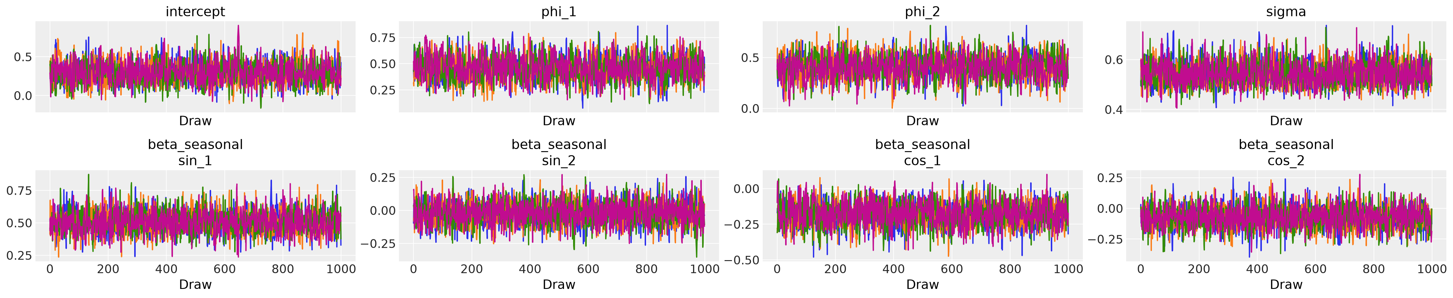
Eight parameters, a deterministic filter, and a survival term. Four chains of 1,000 warmup and 1,000 draws, target_accept=0.9. Sampling is sequential because JAX is already imported; forking the process from a multithreaded JAX runtime is unsafe. The smoke check uses one short chain and does not recover parameters.

SAMPLE_KWARGS = {"target_accept": 0.9, "cores": 1}
censored = HMCForecaster(
    CensoredAR2(),
    train,
    inputs.isel(time=slice(n_train)),
    draws=DRAWS,
    tune=TUNE,
    chains=CHAINS,
    random_seed=SEED,
    progressbar=False,
    sample_kwargs=SAMPLE_KWARGS,
)
assert "eps_future" not in censored.idata.posterior
summary = az.summary(
    censored.idata,
    var_names=["intercept", "phi_1", "phi_2", "sigma", "beta_seasonal"],
)
display(summary)

# compact=True is ArviZ 0.x only; 1.x rejects the keyword.
az.plot_trace(
    censored.idata,
    var_names=["intercept", "phi_1", "phi_2", "sigma", "beta_seasonal"],
)
plt.tight_layout()
plt.show()

Initializing NUTS using jitter+adapt_diag...

Sequential sampling (4 chains in 1 job)

NUTS: [intercept, phi_1, phi_2, sigma, beta_seasonal]

Sampling 4 chains for 1_000 tune and 1_000 draw iterations (4_000 + 4_000 draws total) took 45 seconds.

	mean	sd	hdi94_lb	hdi94_ub	ess_bulk	ess_tail	r_hat	mcse_mean	mcse_sd
intercept	0.295	0.138	0.047	0.56	2039	2150	1.00	0.0031	0.0025
phi_1	0.458	0.113	0.25	0.68	1801	1980	1.00	0.0027	0.0019
phi_2	0.409	0.115	0.2	0.63	1768	2113	1.01	0.0028	0.0019
sigma	0.545	0.047	0.46	0.63	2404	2272	1.00	0.00098	0.00082
beta_seasonal[sin_1]	0.508	0.085	0.34	0.66	2402	2682	1.00	0.0017	0.0014
beta_seasonal[sin_2]	-0.019	0.085	-0.18	0.13	2736	2583	1.00	0.0016	0.0014
beta_seasonal[cos_1]	-0.178	0.084	-0.34	-0.025	2001	2075	1.00	0.0019	0.0012
beta_seasonal[cos_2]	-0.073	0.088	-0.24	0.095	3064	2663	1.00	0.0016	0.0015

/var/folders/cm/3dzy9rdd5s3672z0s1brjkvh0000gn/T/ipykernel_69780/1384402765.py:25: UserWarning: The figure layout has changed to tight
  plt.tight_layout()

../_images/57ce3df476846b476dc97432fba187e87dbd48b21abdf67eb867461557476ef1.png

In-sample bands are demand-scale sales#

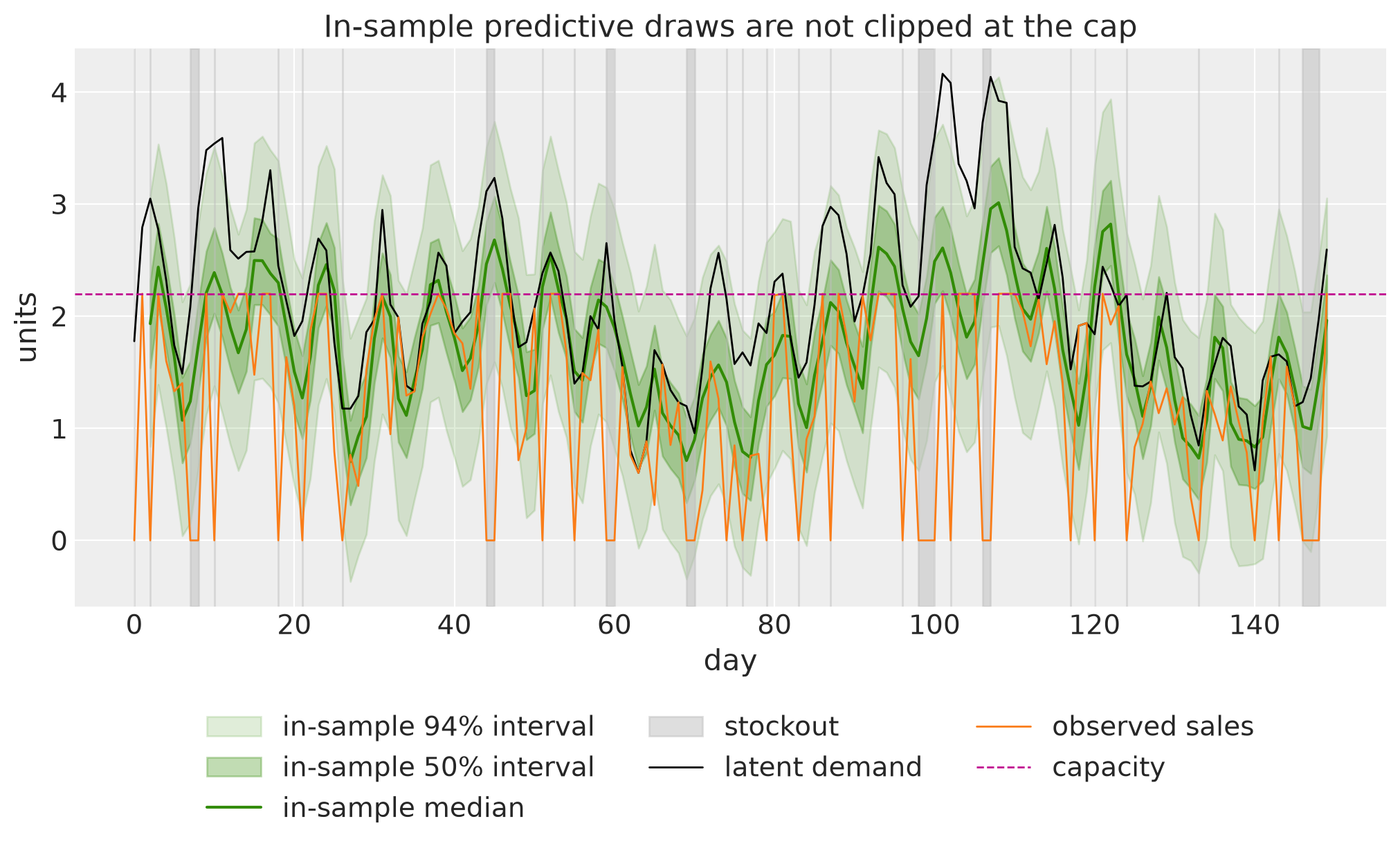
Posterior predictive draws come from the uncensored normal, so they may exceed the cap and dip below zero. That is the point of not using pm.Censored. The first two steps are placeholder lags and are dropped. Gray bands are stockouts: the filter carries the prediction instead of the recorded zero. The black line is latent demand, which the likelihood never saw. Sales sit below it by the friction term.

def central_bands(ax, samples, x, color, label):
    """Plot the median and the central 50% and 94% intervals."""
    stacked = samples.stack(sample=("chain", "draw"))
    quantiles = stacked.quantile([0.03, 0.25, 0.5, 0.75, 0.97], dim="sample")
    x = np.asarray(x)
    band = {q: np.asarray(quantiles.sel(quantile=q)) for q in (0.03, 0.25, 0.5, 0.75, 0.97)}
    ax.fill_between(
        x, band[0.03], band[0.97], color=color, alpha=0.15, label=f"{label} 94% interval"
    )
    ax.fill_between(
        x, band[0.25], band[0.75], color=color, alpha=0.3, label=f"{label} 50% interval"
    )
    ax.plot(x, band[0.5], color=color, lw=1.5, label=f"{label} median")


in_sample = censored.predict_in_sample(posterior=censored.idata, random_seed=SEED + 1)
fig, ax = plt.subplots()
kept = slice(N_ORDER, None)
# obs is the training window; time is the full series, including the horizon.
in_sample_obs = in_sample.posterior_predictive.obs.isel(time=kept)
train_time = time[:n_train][kept]
assert in_sample_obs.sizes["time"] == len(train_time)
central_bands(ax, in_sample_obs, train_time, "C2", "in-sample")
stockout = series["available"][:n_train] == 0
ax.fill_between(
    time[:n_train],
    0,
    1,
    where=stockout,
    transform=ax.get_xaxis_transform(),
    color="0.75",
    alpha=0.5,
    step="mid",
    label="stockout",
)
ax.plot(time[:n_train], series["demand"][:n_train], color="black", lw=1, label="latent demand")
ax.plot(time[:n_train], series["sales_obs"][:n_train], color="C1", lw=1, label="observed sales")
ax.axhline(float(CAPACITY), color="C3", ls="--", lw=1, label="capacity")
ax.legend(loc="upper center", bbox_to_anchor=(0.5, -0.15), ncol=3)
ax.set(title="In-sample predictive draws are not clipped at the cap", xlabel="day", ylabel="units")
plt.show()

Sampling: [obs]

../_images/2ffdd2b80729a0c06db6aa1d3f18357688e43045823fe79dccd10d7ff20008e2.png

Forecast the uncensored scenario#

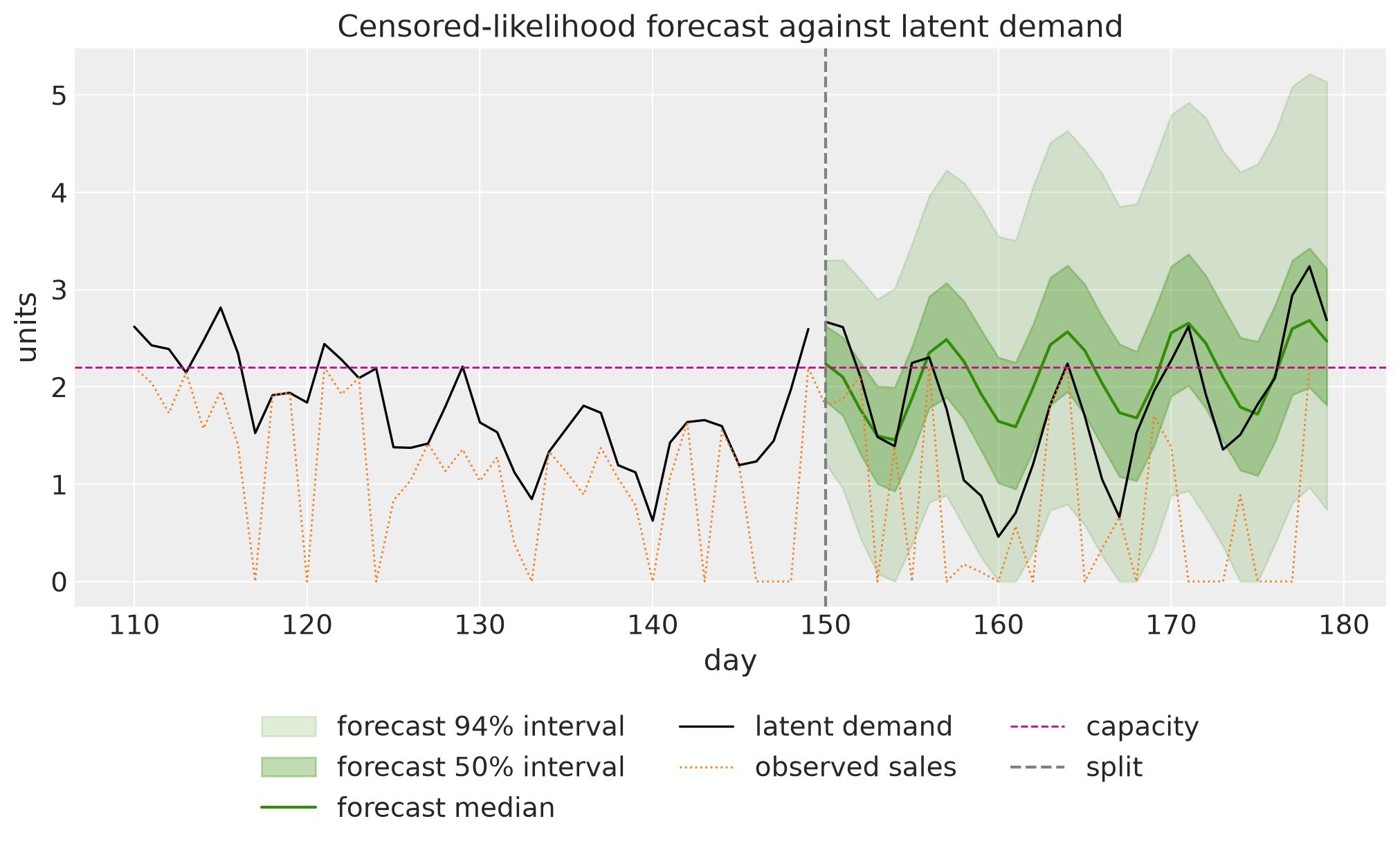
forecast rebuilds the model on the full covariate horizon and draws eps_future from the noise distribution. Those errors are not in the posterior. The registered forecast clips each simulated trajectory at zero. Score it against latent demand, the series the model never saw. Passing posterior=idata uses every MCMC draw. The default of 100 would not be the comparison this notebook is making.

prediction = censored.forecast(covariates=inputs, posterior=censored.idata, random_seed=SEED + 2)
forecast = prediction.predictions.forecast
assert forecast.dims == ("chain", "draw", "time_future")
assert forecast.sizes["time_future"] == HORIZON
demand_future = (
    xr.DataArray(series["demand"], dims="time", coords={"time": time})
    .isel(time=slice(n_train, None))
    .rename(time="time_future")
)
sales_future = sales_obs.isel(time=slice(n_train, None)).rename(time="time_future")
assert np.array_equal(forecast.time_future.values, demand_future.time_future.values)

fig, ax = plt.subplots()
central_bands(ax, forecast, forecast.time_future.values, "C2", "forecast")
history_start = max(0, n_train - 40)
ax.plot(
    time[history_start:n_train],
    series["demand"][history_start:n_train],
    color="black",
    lw=1.2,
    label="latent demand",
)
ax.plot(forecast.time_future.values, demand_future.values, color="black", lw=1.2)
ax.plot(
    time[history_start:],
    series["sales_obs"][history_start:],
    color="C1",
    ls=":",
    lw=1,
    label="observed sales",
)
ax.axhline(float(CAPACITY), color="C3", ls="--", lw=1, label="capacity")
ax.axvline(n_train, color="0.5", ls="--", label="split")
ax.legend(loc="upper center", bbox_to_anchor=(0.5, -0.15), ncol=3)
ax.set(title="Censored-likelihood forecast against latent demand", xlabel="day", ylabel="units")
plt.show()

Sampling: [eps_future]

../_images/8d663160bdbe393dc09c9e8d97cba56286f395f7719d42be4ddf20845aa92bc5.png

The naive model treats the cap as data#

Zero the censoring column and refit. The forecast must be rebuilt on that same tensor. Replaying the naive posterior through the original covariates would filter the training lags with a censoring rule the fit never saw.

naive_inputs = inputs.copy(deep=True)
naive_inputs.loc[{"input": "censored"}] = 0.0
naive = HMCForecaster(
    CensoredAR2(),
    train,
    naive_inputs.isel(time=slice(n_train)),
    draws=DRAWS,
    tune=TUNE,
    chains=CHAINS,
    random_seed=SEED + 3,
    progressbar=False,
    sample_kwargs=SAMPLE_KWARGS,
)
naive_summary = az.summary(
    naive.idata,
    var_names=["intercept", "phi_1", "phi_2", "sigma", "beta_seasonal"],
)
display(naive_summary)

Initializing NUTS using jitter+adapt_diag...

Sequential sampling (4 chains in 1 job)

NUTS: [intercept, phi_1, phi_2, sigma, beta_seasonal]

Sampling 4 chains for 1_000 tune and 1_000 draw iterations (4_000 + 4_000 draws total) took 26 seconds.

	mean	sd	hdi94_lb	hdi94_ub	ess_bulk	ess_tail	r_hat	mcse_mean	mcse_sd
intercept	0.448	0.131	0.21	0.69	3149	2756	1.00	0.0023	0.002
phi_1	0.407	0.095	0.23	0.59	2531	2719	1.00	0.0019	0.0014
phi_2	0.317	0.097	0.13	0.49	2541	2478	1.00	0.0019	0.0015
sigma	0.434	0.0301	0.38	0.49	3369	2693	1.00	0.00052	0.0005
beta_seasonal[sin_1]	0.345	0.059	0.24	0.46	4041	3103	1.00	0.00093	0.00094
beta_seasonal[sin_2]	0.013	0.061	-0.1	0.13	4331	2615	1.00	0.00092	0.001
beta_seasonal[cos_1]	-0.159	0.061	-0.27	-0.041	2962	2410	1.00	0.0011	0.00091
beta_seasonal[cos_2]	-0.086	0.063	-0.2	0.032	4567	2868	1.00	0.00093	0.0011

naive_prediction = naive.forecast(
    covariates=naive_inputs,
    posterior=naive.idata,
    random_seed=SEED + 4,
)
naive_forecast = naive_prediction.predictions.forecast
fig, axes = plt.subplots(nrows=2, sharex=True, sharey=True, figsize=(10, 6), layout="constrained")
for ax, draws, title in (
    (axes[0], forecast, "censored likelihood"),
    (axes[1], naive_forecast, "plain normal likelihood"),
):
    central_bands(ax, draws, draws.time_future.values, "C2", "forecast")
    ax.plot(
        draws.time_future.values,
        demand_future.values,
        color="black",
        lw=1.2,
        label="latent demand",
    )
    ax.axhline(float(CAPACITY), color="C3", ls="--", lw=1, label="capacity")
    ax.set(title=title, ylabel="units")
    ax.legend(loc="upper right")
axes[1].set(xlabel="day")
fig.suptitle("Only the censored model follows demand through the cap")
plt.show()

Sampling: [eps_future]

../_images/65970ca8f4b7210d6898349e3199c54b532e22c2dd5741a9b73b3c28d1857887.png

Evaluation#

Two truths, because they answer different questions. Latent demand is the planning quantity, known here only because the series was simulated. Observed sales are what a transaction table would offer, and they are themselves gated and capped, so a demand forecast is penalized for being right. Coverage is the central interval, not an HDI. On peak days — latent demand above the cap — the naive mean should stay under the cap it mistook for data.

metrics = {
    "mae": eval_mae,
    "rmse": eval_rmse,
    "crps": eval_crps,
    "coverage_50": partial(eval_coverage, alpha=0.5),
    "coverage_94": partial(eval_coverage, alpha=0.94),
}
rows = {
    ("censored likelihood", "latent demand"): evaluate_forecast(
        forecast, demand_future, metrics=metrics
    ),
    ("plain normal likelihood", "latent demand"): evaluate_forecast(
        naive_forecast, demand_future, metrics=metrics
    ),
    ("censored likelihood", "observed sales"): evaluate_forecast(
        forecast, sales_future, metrics=metrics
    ),
    ("plain normal likelihood", "observed sales"): evaluate_forecast(
        naive_forecast, sales_future, metrics=metrics
    ),
}
results = pd.DataFrame(rows).T.round(3)
results.index.names = ["model", "truth"]
display(results)

		mae	rmse	crps	coverage_50	coverage_94
model	truth
censored likelihood	latent demand	0.488	0.639	0.368	0.600	1.000
plain normal likelihood	latent demand	0.490	0.570	0.329	0.467	0.967
censored likelihood	observed sales	1.342	1.631	1.002	0.300	0.600
plain normal likelihood	observed sales	0.993	1.200	0.772	0.300	0.467

peak_times = demand_future.time_future.values[np.asarray(demand_future) > float(CAPACITY)]
print(f"test days with latent demand above the cap: {len(peak_times)} of {HORIZON}")
peak = pd.DataFrame(
    {
        "censored likelihood": evaluate_forecast(
            forecast.sel(time_future=peak_times),
            demand_future.sel(time_future=peak_times),
            metrics=metrics,
        ),
        "plain normal likelihood": evaluate_forecast(
            naive_forecast.sel(time_future=peak_times),
            demand_future.sel(time_future=peak_times),
            metrics=metrics,
        ),
    }
).T.round(3)
peak.index.name = "model"
display(peak)

test days with latent demand above the cap: 10 of 30

	mae	rmse	crps	coverage_50	coverage_94
model
censored likelihood	0.311	0.337	0.270	0.8	1.0
plain normal likelihood	0.688	0.746	0.456	0.3	0.9

censored_mean = forecast.mean(("chain", "draw"))
naive_mean = naive_forecast.mean(("chain", "draw"))
print("censored forecast mean max", float(censored_mean.max()))
print("naive forecast mean max", float(naive_mean.max()))
if not SMOKE:
    published = {"intercept": 0.294, "phi_1": 0.447, "phi_2": 0.419, "sigma": 0.543}
    for name, target in published.items():
        estimate = float(summary.loc[name, "mean"])
        if abs(estimate - target) >= 0.08:
            raise AssertionError(f"{name} mean {estimate:.3f} is not within 0.08 of {target}")
    beta_key = next(idx for idx in summary.index if "sin_1" in str(idx))
    beta_sin = float(summary.loc[beta_key, "mean"])
    if abs(beta_sin - 0.506) >= 0.08:
        raise AssertionError(f"sin_1 coefficient {beta_sin:.3f} is not within 0.08 of 0.506")
    if float(summary.loc["sigma", "mean"]) <= float(naive_summary.loc["sigma", "mean"]) + 0.05:
        raise AssertionError("censored sigma should exceed the naive sigma")
    if float(summary["r_hat"].max()) >= 1.05:
        raise AssertionError(f"r_hat {float(summary['r_hat'].max()):.3f} is at least 1.05")
    censored_peak = float(peak.loc["censored likelihood", "mae"])
    naive_peak = float(peak.loc["plain normal likelihood", "mae"])
    if censored_peak >= naive_peak:
        raise AssertionError("censored peak-day MAE should be lower")
    if float(censored_mean.max()) <= float(CAPACITY) or float(naive_mean.max()) >= float(CAPACITY):
        raise AssertionError("only the censored forecast mean should cross the cap")

censored forecast mean max 2.7887307834947457
naive forecast mean max 2.0218151567476768

What the comparison is saying#

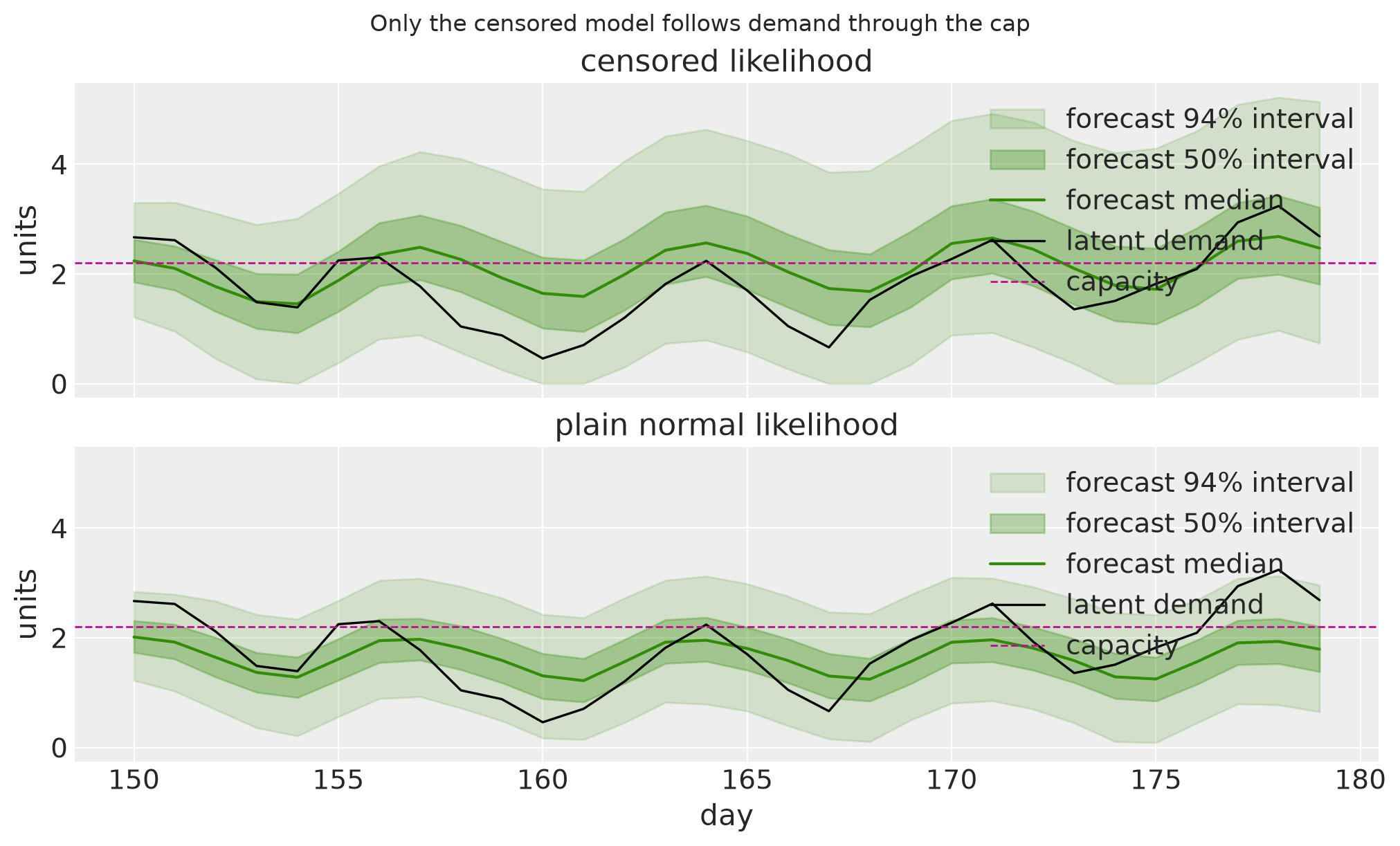
Against latent demand, average point error is close. Both models target the sales scale, which sits below demand by the friction term, and most test days are below the cap. Calibration and the peaks are where the likelihood matters. The censored intervals cover at their nominal level. The naive fit treats every capped day as an exact 2.2, so its mean is pulled down and its \(\sigma\) shrinks. Against observed sales the naive model wins the point scores, and it should: the test register is gated and capped too. Scoring recorded sales rewards a model that repeats the corruption.

On days when latent demand exceeds the cap, the censored forecast follows demand across the line. The naive forecast mean stays under the cap. That is the operational difference.

Example	What the data record	What the model does
Intermittent demand	Occurrence or not	Occurrence times size
Retail stockouts	Availability share	Floored mean factor
This notebook	Cap and off-shelf flag	Survival at the cap

The upstream availability-TSB example freezes a probability recursion on off-shelf days. This package does not include that notebook. The same idea, an update gate plus a masked likelihood, is what ssoe expects the caller to write. The mechanisms compose: a fractional availability factor for partial days, and a survival term where the shelf capacity is known.

Next steps#

Replace \(\max(y_t, \hat{y}_t)\) with the censored conditional mean \(\hat{y}_t + \sigma \varphi(z_t) / (1 - \Phi(z_t))\).
Let the cap vary by day, from inventory. The likelihood already censors at the recorded value, so only the covariate changes.
Use a nonnegative observation distribution so the in-sample bands do not put mass on negative sales.
Replace the single split with backtest, as in the ARMA example.

References#

Orduz, J. Demand Forecasting with Censored Likelihood.
The upstream notebook this example ports.
Tobin, J. (1958). Estimation of Relationships for Limited Dependent Variables. Econometrica, 26(1), 24-36.
NumPyro’s censored distributions.