Exponential smoothing in innovations state-space form#

Damped Holt-Winters smoothing uses one error to update level, trend and seasonality. This notebook uses ssoe to share the training and forecast recursion. The seasonal initial state is centered to separate its average from the initial level. The state is a tuple with two scalars and a seasonal vector.

Based on Juan Orduz’s exponential-smoothing example.

Prepare notebook#

import os

import arviz as az
import matplotlib.pyplot as plt
import numpy as np
import pandas as pd
import pymc as pm
import pytensor.tensor as pt
import xarray as xr

from pymc_forecast import (
    HMCForecaster,
    Horizon,
    evaluate_forecast,
    null_covariates,
    ssoe,
)

SMOKE = os.getenv("PYMC_FORECAST_SMOKE_TEST") == "1"
SEED = 42
rng = np.random.default_rng(SEED)
DRAWS, TUNE, CHAINS = (25, 25, 1) if SMOKE else (600, 800, 2)
N_PRED = 50 if SMOKE else 800
HDI_PROB = 0.94

az.style.use("arviz-darkgrid")
if "stats.ci_kind" in az.rcParams:  # ArviZ 1.x; ArviZ 0.x intervals are always HDI
    az.rcParams["stats.ci_kind"] = "hdi"
az.rcParams["stats.ci_prob"] = HDI_PROB
plt.rcParams["figure.figsize"] = [10, 6]
plt.rcParams["figure.dpi"] = 100
plt.rcParams["figure.facecolor"] = "white"

%config InlineBackend.figure_format = "retina"
print(
    "Execution mode:", "CI smoke check; do not interpret fit quality" if SMOKE else "full example"
)

Execution mode: full example

Generate a seasonal series#

n_seasons = 15
t = np.linspace(0, n_seasons + 1, (n_seasons + 1) * n_seasons)
y = np.cos(2 * np.pi * t) + np.log(t + 1) + 0.2 * rng.normal(size=t.shape)
n_train = int(0.8 * len(y))
series = xr.DataArray(y, dims="time", coords={"time": t})
train = series.isel(time=slice(n_train))
truth = series.isel(time=slice(n_train, None)).rename(time="time_future")
full_covariates = null_covariates(t)

One error updates all state components#

With damped trend \(\phi b\) and the current seasonal value \(s_0\), \(\mu_t=\ell+\phi b+s_0\). The same error updates level by \(\alpha\epsilon\), trend by \(\beta\epsilon\) and seasonality by \(\gamma\epsilon\). We retain the original constraints \(\beta=\alpha\,\beta^*\) and \(\gamma=(1-\alpha)\,\gamma^*\).

Only the helper knows whether it is filtering observed errors or drawing future ones. The model below contains one update function for both operations.

The initial seasonal vector has a ZeroSumNormal prior on a named season dimension. This is an explicit change from the original independent Normal prior: it removes the redundant shift between the initial level and average seasonality. The state-update equations are unchanged.

def exponential_smoothing_ssm(covariates, data=None):
    h = Horizon.from_data(covariates, data)
    alpha = pm.Beta("level_smoothing", 5, 5)
    trend_smoothing = pm.Beta("trend_smoothing", 5, 5)
    seasonal_smoothing = pm.Beta("seasonality_smoothing", 5, 5)
    phi = pm.Beta("phi", 2, 5)
    level = pm.Normal("level_init", float(h.data.values[0]), 1)
    trend = pm.Normal("trend_init", 0, 0.1)
    pm.modelcontext(None).add_coord("season", np.arange(n_seasons))
    seasonality = pm.ZeroSumNormal("seasonality_init", sigma=1, dims="season")
    noise = pm.HalfNormal("noise", 0.5)
    beta = alpha * trend_smoothing
    gamma = (1 - alpha) * seasonal_smoothing

    def mean(state, x, alpha, beta, gamma, phi):
        level, trend, seasonality = state
        return level + phi * trend + seasonality[0]

    def update(state, y, error, x, alpha, beta, gamma, phi):
        level, trend, seasonality = state
        new_season = seasonality[0] + gamma * error
        return (
            level + phi * trend + alpha * error,
            phi * trend + beta * error,
            pt.concatenate([seasonality[1:], new_season[None]]),
        )

    r = ssoe(
        h,
        "eps",
        None,
        (level, trend, seasonality),
        mean,
        update,
        pm.Normal.dist(0, noise),
        params=(alpha, beta, gamma, phi),
    )
    pm.Normal("obs", r.mu, noise, observed=h.data.values, dims="time")
    pm.Deterministic("mu", r.mu, dims="time")
    if h.future:
        pm.Deterministic("mu_future", r.mu_future, dims="time_future")
        pm.Deterministic("forecast", r.y_future, dims="time_future")

Fit with NUTS#

fc = HMCForecaster(
    exponential_smoothing_ssm,
    train,
    draws=DRAWS,
    tune=TUNE,
    chains=CHAINS,
    random_seed=SEED,
    progressbar=False,
    sample_kwargs={"target_accept": 0.95},
)
az.summary(
    fc.idata,
    var_names=[
        "level_smoothing",
        "trend_smoothing",
        "seasonality_smoothing",
        "phi",
        "noise",
        "level_init",
        "trend_init",
        "seasonality_init",
    ],
)

Initializing NUTS using jitter+adapt_diag...

Multiprocess sampling (2 chains in 2 jobs)

NUTS: [level_smoothing, trend_smoothing, seasonality_smoothing, phi, level_init, trend_init, seasonality_init, noise]

Sampling 2 chains for 800 tune and 600 draw iterations (1_600 + 1_200 draws total) took 6 seconds.

We recommend running at least 4 chains for robust computation of convergence diagnostics

The rhat statistic is larger than 1.01 for some parameters. This indicates problems during sampling. See https://arxiv.org/abs/1903.08008 for details

	mean	sd	hdi94_lb	hdi94_ub	ess_bulk	ess_tail	r_hat	mcse_mean	mcse_sd
level_smoothing	0.317	0.064	0.2	0.45	1219	682	1.00	0.0019	0.0023
trend_smoothing	0.472	0.146	0.23	0.76	1865	916	1.00	0.0034	0.0037
seasonality_smoothing	0.219	0.069	0.098	0.35	655	724	1.00	0.0026	0.0017
phi	0.192	0.118	0.0043	0.4	1396	869	1.00	0.0031	0.0037
noise	0.2151	0.0121	0.19	0.24	1254	951	1.00	0.00034	0.00032
level_init	0.175	0.158	-0.13	0.47	1760	934	1.00	0.0038	0.0043
trend_init	0.003	0.102	-0.2	0.18	1908	769	1.00	0.0023	0.0032
seasonality_init[0]	0.941	0.099	0.76	1.1	2103	978	1.00	0.0021	0.0031
seasonality_init[1]	0.765	0.1	0.56	0.94	2485	995	1.00	0.002	0.0033
seasonality_init[2]	0.528	0.105	0.33	0.72	1767	934	1.00	0.0025	0.0033
seasonality_init[3]	0.307	0.101	0.13	0.51	1857	776	1.00	0.0024	0.0036
seasonality_init[4]	-0.252	0.096	-0.42	-0.056	2567	925	1.00	0.0019	0.0035
seasonality_init[5]	-0.559	0.101	-0.74	-0.37	2307	894	1.00	0.0021	0.0038
seasonality_init[6]	-0.874	0.098	-1	-0.68	1814	806	1.00	0.0023	0.0036
seasonality_init[7]	-1.034	0.101	-1.2	-0.82	1839	770	1.01	0.0024	0.0037
seasonality_init[8]	-0.944	0.099	-1.1	-0.74	1528	665	1.00	0.0025	0.0032
seasonality_init[9]	-0.773	0.106	-0.98	-0.6	1769	959	1.00	0.0025	0.0029
seasonality_init[10]	-0.362	0.104	-0.55	-0.17	1972	837	1.00	0.0024	0.0032
seasonality_init[11]	0.062	0.1	-0.12	0.25	2124	950	1.01	0.0022	0.0031
seasonality_init[12]	0.441	0.104	0.25	0.64	1790	741	1.00	0.0025	0.0033
seasonality_init[13]	0.799	0.099	0.62	0.98	1756	919	1.00	0.0024	0.0035
seasonality_init[14]	0.955	0.095	0.78	1.1	2183	772	1.00	0.002	0.0033

Forecast and evaluate#

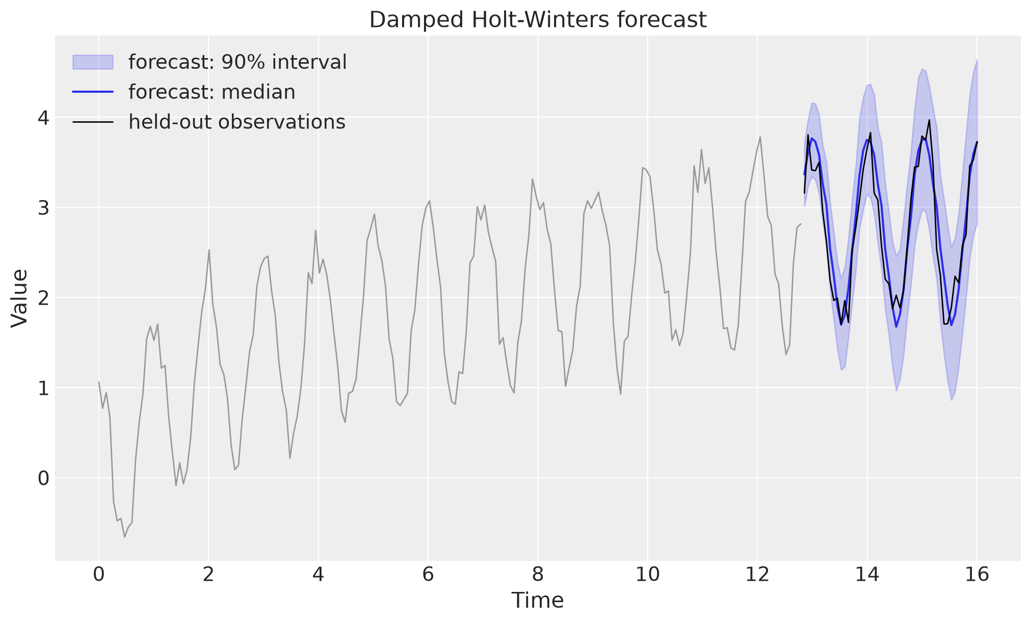
The real-valued time grid is retained by supplying full-horizon covariates. forecast already includes future observation noise; mu_future excludes the current error but retains uncertainty transmitted through earlier future states.

posterior = fc.draw_posterior(N_PRED, random_seed=SEED + 1)
pred = fc.forecast(full_covariates, posterior=posterior, random_seed=SEED + 2).predictions
in_sample = fc.predict_in_sample(posterior=posterior, random_seed=SEED + 3)
np.testing.assert_allclose(pred.forecast - pred.mu_future, pred.eps_future)
assert pred.forecast.sizes["time_future"] == len(truth)
pd.Series(evaluate_forecast(pred.forecast, truth))

Sampling: [eps_future]

Sampling: [obs]

mae         0.202189
rmse        0.251458
crps        0.157586
coverage    1.000000
dtype: float64

def plot_forecast(ax, samples, truth, label="forecast", color="C0"):
    time = samples.time_future.values
    q = samples.quantile([0.05, 0.5, 0.95], dim=("chain", "draw"))
    ax.fill_between(
        time,
        q.sel(quantile=0.05),
        q.sel(quantile=0.95),
        alpha=0.2,
        color=color,
        label=f"{label}: 90% interval",
    )
    ax.plot(time, q.sel(quantile=0.5), color=color, label=f"{label}: median")
    ax.plot(time, truth.values, color="black", lw=1, label="held-out observations")
    ax.set(xlabel="Date", ylabel="Value")
    ax.legend(loc="upper left")

fig, ax = plt.subplots()
plot_forecast(ax, pred.forecast, truth)
ax.plot(train.time, train, color="0.6", lw=1, label="training observations")
ax.set(title="Damped Holt-Winters forecast", xlabel="Time")
plt.show()

../_images/8e028d9aa44d7a560c85a0955d1de638a99a5adf3459e77b364d380ac66dbe78.png

Interpretation#

This example has an observation-driven state with no independently sampled in-sample state path. The separate local-level comparison explains when a latent state and Kalman-filter marginalization are appropriate. The ARMA example provides a smaller introduction to the same ssoe API.