Hierarchical forecasting with pymc_forecast#
This notebook ports the upstream NumPyro hierarchical forecasting example (itself a port
of Pyro’s Forecasting III: hierarchical models)
to the PyMC API. It generalizes the
univariate notebook from a single series to a panel: we
forecast hourly BART arrivals to one destination (EMBR, Embarcadero) from all 50
origin stations at once.
Each origin keeps its own random-walk level, its own weekly seasonal profile, and its
own drift and observation scales — with hyperpriors pooling all of them across
stations. Where the NumPyro version expresses the hierarchy with numpyro.plate,
here the batch structure is a named dim: latents carry dims=("origin",), and
every result comes back as a labeled (time, origin) array.
Prepare notebook#
import logging
import os

import arviz as az
import matplotlib.pyplot as plt
import numpy as np
import pymc as pm
import pytensor.tensor as pt

from pymc_forecast import (
    Forecaster,
    ForecastingModel,
    build_model,
    eval_crps,
    evaluate_forecast,
    null_covariates,
    periodic_repeat,
)
from pymc_forecast.data import FUTURE_DIM, TIME_DIM
from pymc_forecast.datasets import load_bart_od

HDI_PROB = 0.94

az.style.use("arviz-darkgrid")
az.rcParams["stats.ci_kind"] = "hdi"
az.rcParams["stats.ci_prob"] = HDI_PROB
plt.rcParams["figure.figsize"] = [10, 6]
plt.rcParams["figure.dpi"] = 100
plt.rcParams["figure.facecolor"] = "white"

%config InlineBackend.figure_format = "retina"

logging.getLogger("pymc").setLevel(logging.ERROR)
logging.getLogger("pytensor").setLevel(logging.ERROR)

SEED = 42

# CI executes every example notebook end-to-end with reduced settings.
SMOKE_TEST = os.environ.get("PYMC_FORECAST_SMOKE_TEST", "0") == "1"
NUM_STEPS = 200 if SMOKE_TEST else 25_000
NUM_SAMPLES = 50 if SMOKE_TEST else 500
Read data#
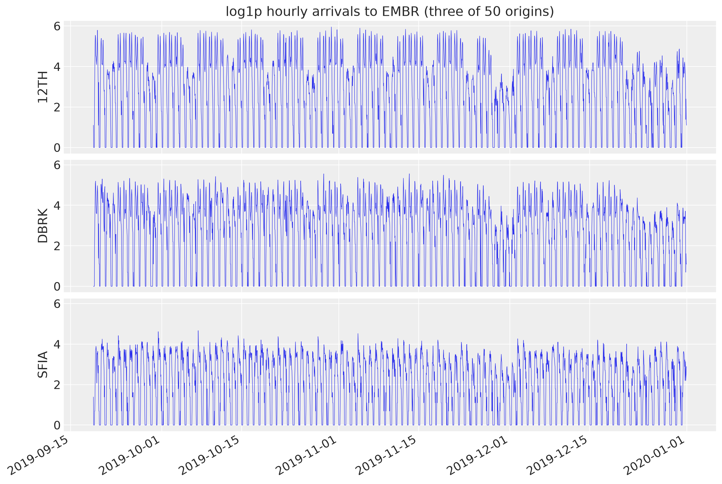
We window the complete hourly origin-destination panel to the last 90 training days plus
two test weeks, select arrivals to EMBR from every origin, and apply log1p — it tames
the multiplicative daily swings while staying defined at zero rides. The result is a
labeled (time, origin) array.
PERIOD = 24 * 7
TRAIN_DAYS = 90
TEST_HOURS = 2 * PERIOD
WINDOW = TRAIN_DAYS * 24 + TEST_HOURS

od = load_bart_od()
arrivals = od.sel(destination="EMBR").isel({TIME_DIM: slice(-WINDOW, None)})
y = np.log1p(arrivals.astype("float64"))
time_values = y[TIME_DIM].values
print("panel:", dict(y.sizes))
print("window:", time_values[0], "->", time_values[-1])
panel: {'time': 2496, 'origin': 50}
window: 2019-09-19T00:00:00 -> 2019-12-31T23:00:00
SHOW_ORIGINS = ["12TH", "DBRK", "SFIA"]

fig, axes = plt.subplots(len(SHOW_ORIGINS), 1, figsize=(12, 8), sharex=True, sharey=True)
for ax, origin in zip(axes, SHOW_ORIGINS, strict=True):
    series = y.sel(origin=origin)
    ax.plot(time_values, series.values, lw=0.5, color="C0")
    ax.set_ylabel(origin)
axes[0].set_title("log1p hourly arrivals to EMBR (three of 50 origins)")
fig.autofmt_xdate()
plt.show()
Train-test split#
Hold out the last two weeks (336 hours) for testing.
y_train = y.isel({TIME_DIM: slice(None, -TEST_HOURS)})
y_test = y.isel({TIME_DIM: slice(-TEST_HOURS, None)})
print("train:", dict(y_train.sizes), "test:", dict(y_test.sizes))
train: {'time': 2160, 'origin': 50} test: {'time': 336, 'origin': 50}
Model specification#
This is the univariate local-level model lifted to a panel, with partial pooling. Each origin \(s\) gets its own random-walk level \(\ell_{t,s}\), its own weekly seasonal profile (one value per hour-of-week, 168 per origin), its own drift scale, and its own observation scale — and every per-origin quantity is drawn from a shared hyperprior, which is what lets quiet stations borrow strength from busy ones:
Three things carry the hierarchy in pymc_forecast:
innovations(..., dims=("origin",))samples the drift once per time step per origin — and creates the matchingdrift_raw_futurevariable with the same batch dim on the forecast horizon.Each origin’s weekly profile is pooled toward a shared profile \(m\) (non-centered, which keeps mean-field ADVI happy), registered on a coord the model body adds itself, then tiled over the horizon with
periodic_repeat.The per-origin scales are
LogNormalvariables whose location and spread are themselves learned hyperparameters.
The "origin" coord itself is registered automatically from the data’s non-time dims.
class HierarchicalLocalLevel(ForecastingModel):
    """Per-origin local level + weekly seasonality, partially pooled across origins."""

    def model(self, covariates, data=None) -> None:
        h = self.horizon
        model = pm.modelcontext(None)
        model.add_coord("hour_of_week", np.arange(PERIOD))
        n_origin = len(model.coords["origin"])

        # per-origin drift and observation scales, pooled through hyperpriors
        drift_loc = pm.Normal("drift_scale_loc", -20.0, 5.0)
        drift_spread = pm.HalfNormal("drift_scale_spread", 1.0)
        drift_scale = pm.LogNormal(
            "drift_scale",
            drift_loc,
            drift_spread,
            dims=("origin",),
            initval=np.full(n_origin, 0.01),
        )
        sigma_loc = pm.Normal("sigma_loc", -5.0, 5.0)
        sigma_spread = pm.HalfNormal("sigma_spread", 1.0)
        sigma = pm.LogNormal(
            "sigma",
            sigma_loc,
            sigma_spread,
            dims=("origin",),
            initval=np.full(n_origin, 0.05),
        )

        # per-origin weekly profile pooled toward a shared profile (non-centered)
        seasonal_mu = pm.Normal("seasonal_mu", 0.0, 5.0, dims=("hour_of_week",))
        seasonal_spread = pm.HalfNormal("seasonal_spread", 2.0)
        seasonal_z = pm.Normal("seasonal_z", 0.0, 1.0, dims=("hour_of_week", "origin"))
        seasonal = seasonal_mu[:, None] + seasonal_spread * seasonal_z

        drift_raw = self.innovations("drift_raw", pm.Normal.dist(0.0, 1.0), dims=("origin",))
        level = pt.cumsum(drift_raw * drift_scale, axis=0)
        prediction = level + periodic_repeat(seasonal, h.duration, axis=0, period=PERIOD)

        self.predict(
            lambda name, mu, dims, observed: pm.Normal(
                name, mu, sigma, dims=dims, observed=observed
            ),
            prediction,
        )


model = HierarchicalLocalLevel()
build_model(model, y_train, null_covariates(y_train[TIME_DIM].values))
Inference with ADVI#
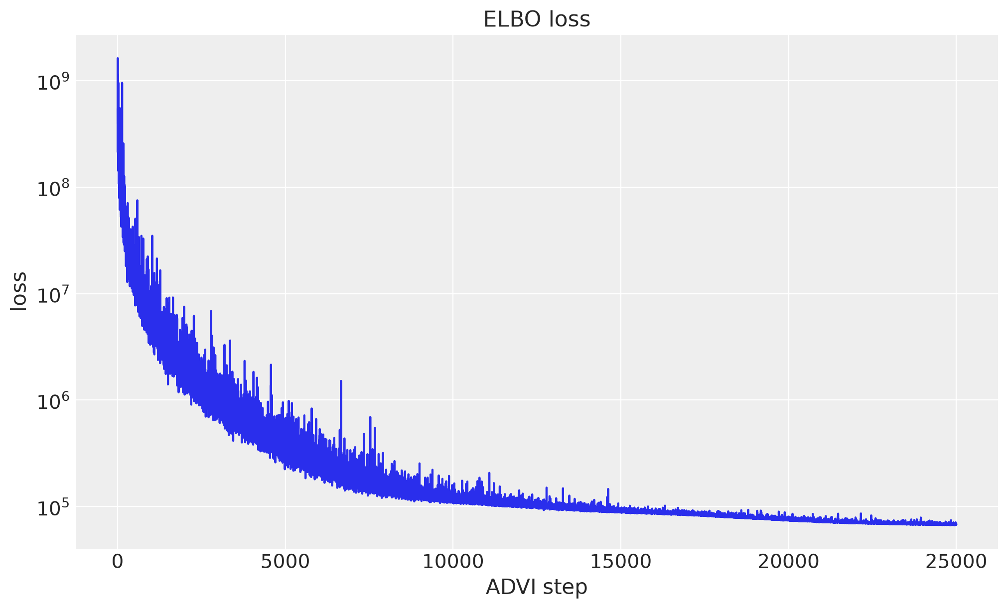
The model has one latent per hour per origin (plus 168 seasonal values per origin), about 120k parameters in total — routine for mean-field ADVI. The model learns seasonality from the time index alone, so no covariates are needed anywhere.
forecaster = Forecaster(
    model,
    y_train,
    optimizer=0.01,
    num_steps=NUM_STEPS,
    random_seed=SEED,
)

fig, ax = plt.subplots()
ax.plot(forecaster.losses)
ax.set(title="ELBO loss", xlabel="ADVI step", ylabel="loss", yscale="log")
plt.show()
/Users/juanitorduz/.paseo/worktrees/1dtaxlkh/docs-example-notebook-visual-style/pymc_forecast/fit.py:251: UserWarning: ADVI has not converged after 25000 steps: the ELBO loss is still descending (median over the last 2500 steps improved by 2.65e+04 since mid-run, more than the within-window fluctuation 718). The forecast may be confidently wrong — increase num_steps, raise the learning rate, or use HMCForecaster; inspect the loss history via the `losses` attribute.
  _check_vi_convergence(losses, num_steps)
Forecast and evaluation#
For a covariate-free model, horizon= extends the training index at its own spacing.
The forecast comes back with dims (chain, draw, time_future, origin), and
evaluate_forecast aligns prediction and truth by dim name — the same call as in
the univariate case, now scoring all 50 series at once.
forecast_idata = forecaster.forecast(
    horizon=TEST_HOURS,
    num_samples=NUM_SAMPLES,
    random_seed=SEED,
)
forecast = forecast_idata["predictions"]["forecast"]
print("forecast dims:", dict(forecast.sizes))

truth = y_test.rename({TIME_DIM: FUTURE_DIM})
print("test:", evaluate_forecast(forecast, truth))
forecast dims: {'chain': 1, 'draw': 500, 'time_future': 336, 'origin': 50}
test: {'mae': 0.4746775267302424, 'rmse': 0.8165881863922577, 'crps': 0.38005588173617105, 'coverage': 0.8207738095238095}
Per-origin scores#
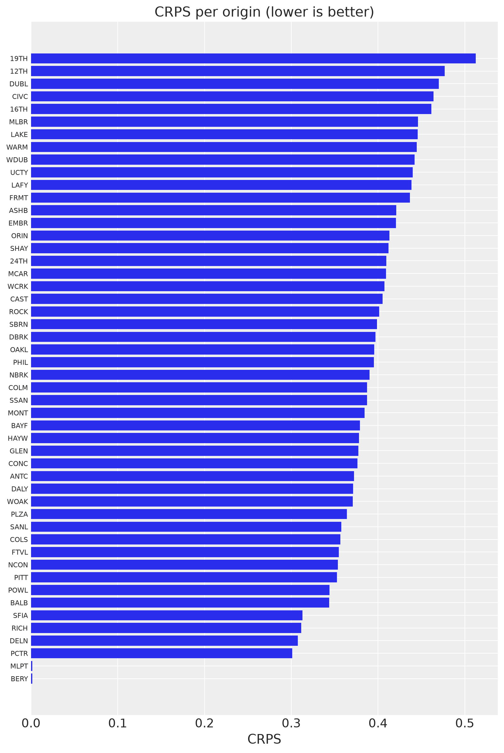
Because everything is labeled, per-series diagnostics are one sel away: score each
origin separately and see where the pooled model does well or poorly.
per_origin = {
    str(origin): eval_crps(forecast.sel(origin=origin), truth.sel(origin=origin))
    for origin in y["origin"].values
}
crps_sorted = sorted(per_origin.items(), key=lambda kv: kv[1])

fig, ax = plt.subplots(figsize=(8, 12))
names = [name for name, _ in crps_sorted]
values = [value for _, value in crps_sorted]
ax.barh(names, values, color="C0")
ax.set(title="CRPS per origin (lower is better)", xlabel="CRPS")
ax.tick_params(axis="y", labelsize=8)
plt.show()
The pooled scales#
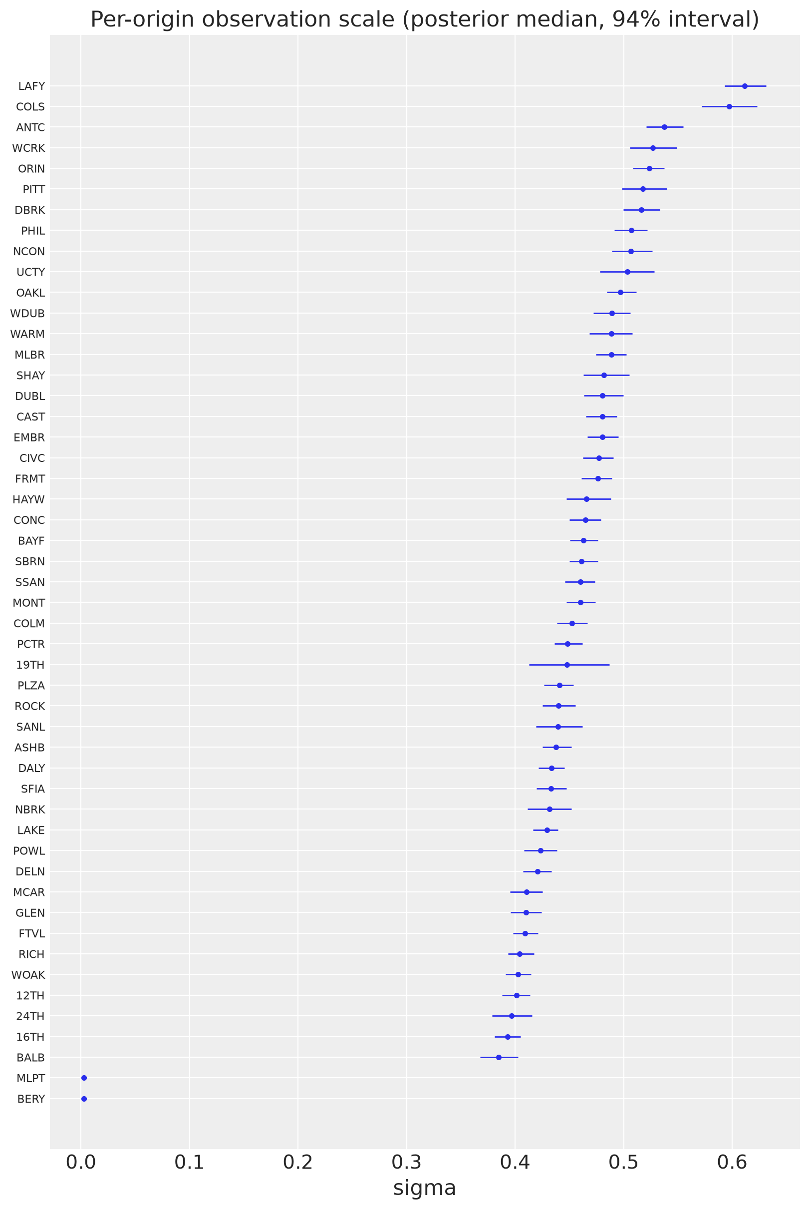
The hyperpriors let each origin keep its own noise level while shrinking all of them toward a common center. Plotting the per-origin posterior observation scales against each station’s forecast difficulty makes the pooling visible: the scales vary smoothly over roughly one order of magnitude rather than scattering to extremes.
posterior = forecaster.draw_posterior(NUM_SAMPLES, random_seed=SEED)
sigma_quantiles = posterior["sigma"].quantile([0.03, 0.5, 0.97], dim=("chain", "draw"))
order = sigma_quantiles.sel(quantile=0.5).argsort().values

fig, ax = plt.subplots(figsize=(8, 12))
positions = np.arange(len(order))
ax.errorbar(
    sigma_quantiles.sel(quantile=0.5).values[order],
    positions,
    xerr=np.stack(
        [
            (sigma_quantiles.sel(quantile=0.5) - sigma_quantiles.sel(quantile=0.03)).values[order],
            (sigma_quantiles.sel(quantile=0.97) - sigma_quantiles.sel(quantile=0.5)).values[order],
        ]
    ),
    fmt="o",
    color="C0",
    ecolor="C0",
    elinewidth=1,
    markersize=3,
)
ax.set_yticks(positions)
ax.set_yticklabels(posterior["origin"].values[order], fontsize=8)
ax.set(title="Per-origin observation scale (posterior median, 94% interval)", xlabel="sigma")
plt.show()
Forecast visualization#
def plot_band(ax, samples, dim, color, label):
    """Median line and 50% / 94% quantile bands of a (chain, draw, time) array."""
    time_axis = samples[dim].values
    quantiles = samples.quantile([0.03, 0.25, 0.5, 0.75, 0.97], dim=("chain", "draw"))
    ax.fill_between(
        time_axis,
        quantiles.sel(quantile=0.03),
        quantiles.sel(quantile=0.97),
        color=color,
        alpha=0.2,
        label=f"{label} 94%",
    )
    ax.fill_between(
        time_axis,
        quantiles.sel(quantile=0.25),
        quantiles.sel(quantile=0.75),
        color=color,
        alpha=0.4,
        label=f"{label} 50%",
    )
    ax.plot(time_axis, quantiles.sel(quantile=0.5), color=color, lw=1)


ZOOM_HOURS = TEST_HOURS + PERIOD

fig, axes = plt.subplots(len(SHOW_ORIGINS), 1, figsize=(12, 10), sharex=True)
for ax, origin in zip(axes, SHOW_ORIGINS, strict=True):
    plot_band(ax, forecast.sel(origin=origin), FUTURE_DIM, "C1", "forecast")
    zoom = y.sel(origin=origin).isel({TIME_DIM: slice(-ZOOM_HOURS, None)})
    ax.plot(zoom[TIME_DIM].values, zoom.values, color="black", lw=0.5, label="observed")
    ax.axvline(truth[FUTURE_DIM].values[0], color="gray", ls="--")
    ax.set_ylabel(f"{origin} (CRPS {per_origin[origin]:.2f})")
axes[0].set_title("Two-week forecasts, arrivals to EMBR")
axes[-1].legend(loc="upper center", bbox_to_anchor=(0.5, -0.25), ncol=3)
fig.autofmt_xdate()
plt.show()
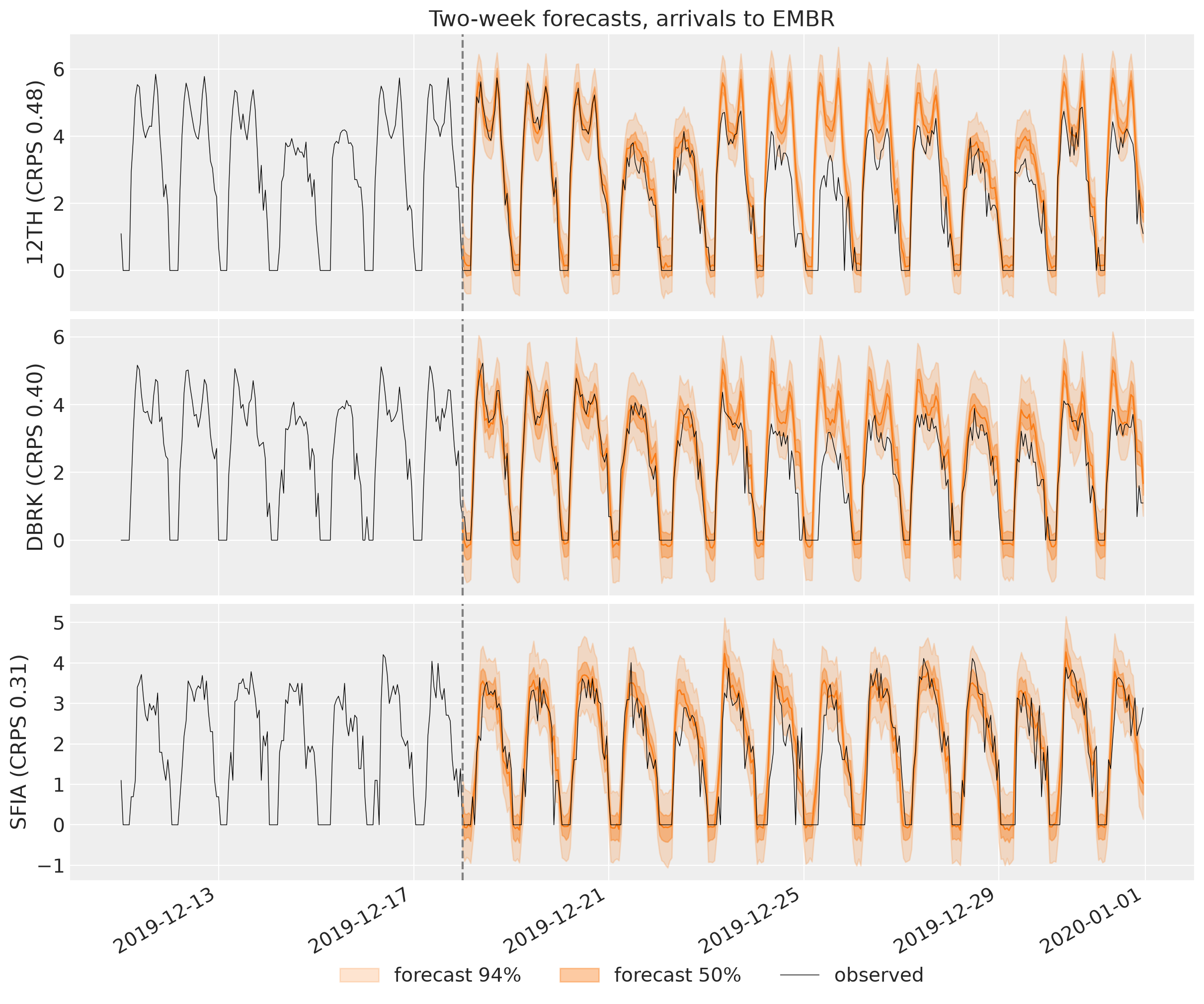
The pooled model tracks each origin’s own weekly rhythm — commuter-heavy stations keep their sharp weekday double peak, quieter ones their flatter profile — while the hyperpriors keep every per-origin scale and seasonal profile regularized toward the panel-wide behavior.
References#
Upstream NumPyro notebook: juanitorduz/numpyro_forecast
Juan Orduz, Hierarchical forecasting with NumPyro (part I): https://juanitorduz.github.io/numpyro_hierarchical_forecasting_1/
Pyro, Forecasting III: hierarchical models: https://pyro.ai/examples/forecasting_iii.html