Forecasting retail demand under stockouts

A store cannot sell what is not on the shelf: recorded sales are a censored version of demand. A model that ignores this reads every stockout dip as a demand drop and under-forecasts exactly the products a planner most needs to reorder. This notebook ports Juan Orduz’s Forecasting Retail Demand Under Stockouts (built on numpyro_forecast) to pymc_forecast (issue #47).

We model daily demand for a panel of store-product series from FreshRetailNet-50K — 50,000 series with hourly stockout labels — with:

• a hierarchical damped-trend model: per-series random-walk level, damped AR(1) slope (a markov_time_series scan latent), weekly seasonality, and promotion covariates pooled by store;

• a floored saturating availability factor that multiplies expected sales: at full availability it is exactly 1, at zero recorded availability it falls to a learned floor rather than 0 — because a small share of sales happens even on days flagged fully out of stock (label noise the data itself reveals below);

• a counterfactual demand forecast: replaying the forecast with availability pinned to 1 turns the sales model into the unconstrained-demand estimate planners should order against.

The upstream example fits all 50,000 series with SVI on a GPU in about six minutes. Here we fit a reduced panel — the top products of the highest-volume stores — with the JAX ADVI backend (Forecaster(..., backend="jax")), which runs on CPU anywhere and on GPU wherever a CUDA JAX is installed; the closing section explains what changes at full scale.

Prepare notebook

import logging
import os

import arviz as az
import jax
import matplotlib.pyplot as plt
import numpy as np
import pandas as pd
import polars as pl
import pooch
import pymc as pm
import pytensor
import pytensor.tensor as pt
import xarray as xr

from pymc_forecast import (
    Forecaster,
    ForecastingModel,
    Horizon,
    build_model,
    eval_coverage,
    eval_crps,
)
from pymc_forecast.data import FUTURE_DIM, TIME_DIM

az.style.use("arviz-darkgrid")
plt.rcParams["figure.figsize"] = [10, 6]
plt.rcParams["figure.dpi"] = 100
plt.rcParams["figure.facecolor"] = "white"

logging.getLogger("pymc").setLevel(logging.ERROR)
logging.getLogger("pytensor").setLevel(logging.ERROR)

SEED = 42

# CI executes every example notebook end-to-end with reduced settings.
SMOKE_TEST = os.environ.get("PYMC_FORECAST_SMOKE_TEST", "0") == "1"
N_STORES = 4 if SMOKE_TEST else 10
N_PER_STORE = 10 if SMOKE_TEST else 20
NUM_STEPS = 200 if SMOKE_TEST else 40_000
NUM_SAMPLES = 50 if SMOKE_TEST else 200
POSTERIOR_BATCH_SIZE = 50
PREDICTIVE_BATCH_SIZE = 50

T_TRAIN = 76
HORIZON = 14

print(f"JAX devices: {jax.devices()}")

JAX devices: [CpuDevice(id=0)]

Read data

FreshRetailNet-50K ships 90 days (2024-03-28 to 2024-06-25) of daily store-product rows with hourly sales, hourly stockout flags, and promotion covariates. The single training parquet holds 4.5 million rows, so we scan it lazily with polars and only ever collect aggregates. The download (~100 MB) is cached by pooch.

parquet_path = pooch.retrieve(
    url="https://huggingface.co/datasets/Dingdong-Inc/FreshRetailNet-50K/resolve/main/data/train.parquet",
    known_hash="sha256:6706832db892bbae4969c19d87e07975d2543d2ba7d7d4756360654785de5a3d",
    fname="fresh_retail_train.parquet",
    path=pooch.os_cache("pymc_forecast"),
    progressbar=False,
)
data_lf = pl.scan_parquet(parquet_path)

data_lf.select(
    pl.len().alias("rows"),
    pl.col("store_id").n_unique().alias("stores"),
    pl.col("product_id").n_unique().alias("products"),
    pl.struct(["store_id", "product_id"]).n_unique().alias("series"),
    pl.col("dt").min().alias("start_date"),
    pl.col("dt").max().alias("end_date"),
).collect(engine="streaming")

shape: (1, 6)

rows	stores	products	series	start_date	end_date
u32	u32	u32	u32	str	str
4500000	898	865	50000	"2024-03-28"	"2024-06-25"

How bad is the stockout problem?

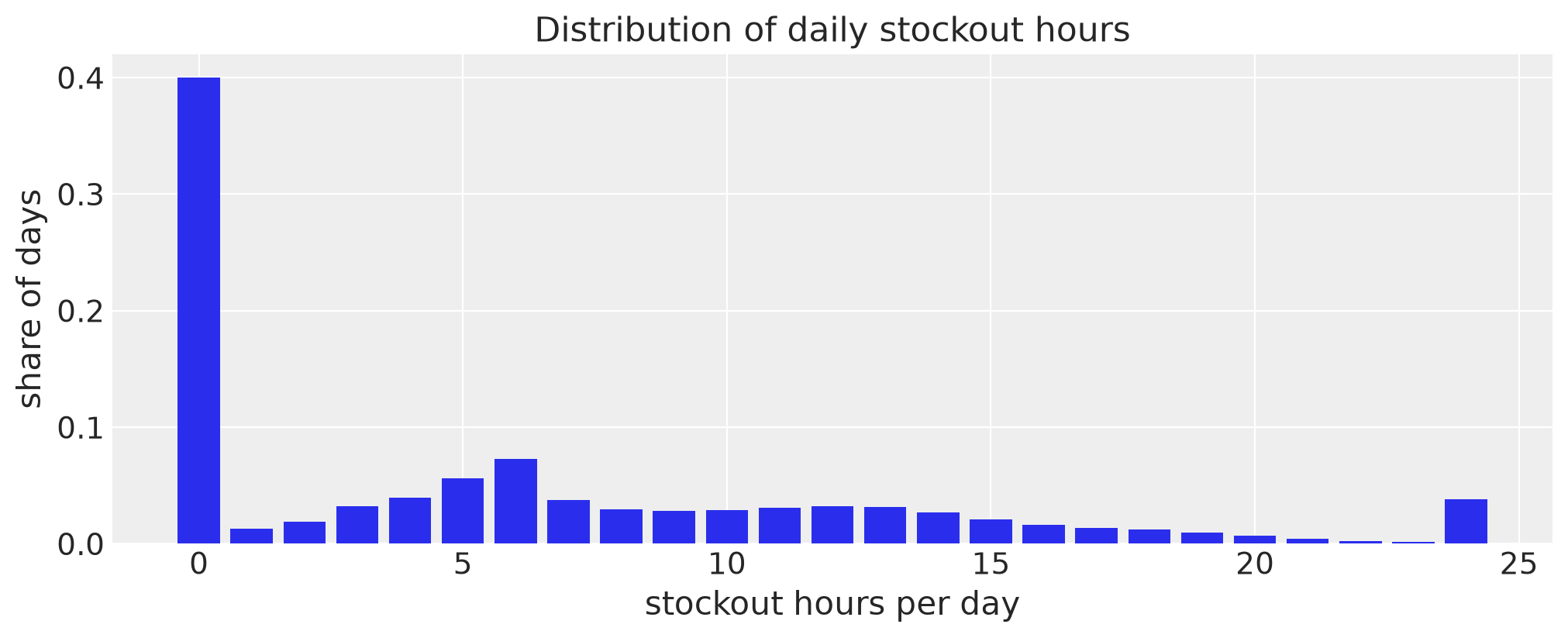
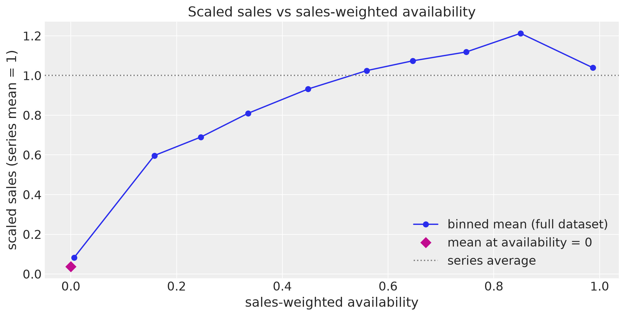
Three facts drive the model design. First, stockouts are pervasive — most days lose at least a few hours of shelf time. Second, hours are not equal: almost all sales happen between 6:00 and 22:00, so an availability measure should weight each hour by its share of sales. Third — and this is the key one — the stockout labels are noisy: a meaningful share of days flagged out of stock for all 24 hours still records positive sales. Hard-censoring sales to zero at zero availability would contradict the data; the model needs a floor.

stockout_hours = pl.col("hours_stock_status").list.sum()

stockout_hours_df = (
    data_lf.group_by(stockout_hours.alias("stockout_hours"))
    .len()
    .sort("stockout_hours")
    .with_columns((pl.col("len") / pl.col("len").sum()).alias("share_of_days"))
    .collect(engine="streaming")
)

fig, ax = plt.subplots(figsize=(10, 4))
ax.bar(stockout_hours_df["stockout_hours"], stockout_hours_df["share_of_days"], color="C0")
ax.set(
    xlabel="stockout hours per day",
    ylabel="share of days",
    title="Distribution of daily stockout hours",
)
plt.show()

hourly_row = (
    data_lf.select(
        *[pl.col("hours_sale").list.get(h).sum().alias(f"sales_{h}") for h in range(24)],
        *[pl.col("hours_stock_status").list.get(h).mean().alias(f"oos_{h}") for h in range(24)],
    )
    .collect(engine="streaming")
    .row(0)
)
sales_by_hour = np.asarray(hourly_row[:24], dtype=np.float64)
stockout_rate_by_hour = np.asarray(hourly_row[24:], dtype=np.float64)
hourly_weights = sales_by_hour / sales_by_hour.sum()

fig, ax = plt.subplots(figsize=(10, 4))
ax.bar(np.arange(24), hourly_weights, color="C0", alpha=0.8, label="share of daily sales")
ax_twin = ax.twinx()
ax_twin.plot(np.arange(24), stockout_rate_by_hour, "o-", color="C1", label="stockout rate")
ax_twin.grid(False)
ax_twin.set(ylabel="stockout rate", ylim=(0, 0.5))
handles, labels = ax.get_legend_handles_labels()
handles_twin, labels_twin = ax_twin.get_legend_handles_labels()
ax.legend(handles + handles_twin, labels + labels_twin, loc="upper left")
ax.set(xlabel="hour of day", ylabel="share of daily sales", title="Hourly sales vs stockouts")
print(f"share of sales in the 6:00-22:00 window: {hourly_weights[6:22].sum():.1%}")
plt.show()

share of sales in the 6:00-22:00 window: 95.2%

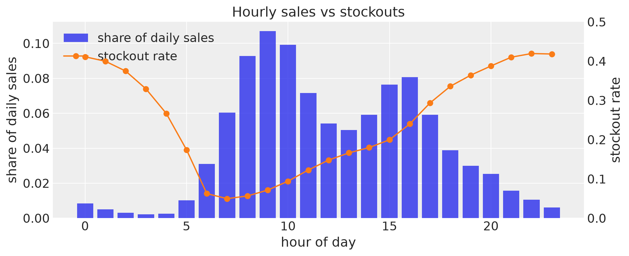
The sales-weighted availability of a day weights each in-stock hour by its share of global sales, so losing the 3 a.m. hour barely moves it while losing the evening peak does:

$$a_{t,s} = \sum_{h=0}^{23} w_h , (1 - \text{stockout}_{t,s,h}), \qquad w_h = \frac{\text{global sales in hour } h}{\text{total global sales}}.$$

Binning all 4.5M day-rows by this availability and averaging each series’ scaled sales (each series divided by its own mean, so 1 is an average day) traces the curve the model must reproduce — including its most awkward feature: the mean scaled sales at zero availability is clearly positive.

def sales_weighted_availability(weights):
    """In-stock share of the day, each hour weighted by its share of global sales."""
    return pl.sum_horizontal(
        [(1 - pl.col("hours_stock_status").list.get(h)) * float(weights[h]) for h in range(24)]
    ).alias("availability")


scaled_sales = pl.col("sale_amount") / pl.col("sale_amount").mean().over("store_id", "product_id")
availability_sales_lf = data_lf.with_columns(
    sales_weighted_availability(hourly_weights), scaled_sales.alias("scaled_sales")
)
factor_curve_df = (
    availability_sales_lf.group_by(
        (pl.col("availability") * 10).floor().clip(0, 9).alias("availability_bin")
    )
    .agg(
        pl.col("availability").mean().alias("mean_availability"),
        pl.col("scaled_sales").mean().alias("mean_scaled_sales"),
    )
    .sort("availability_bin")
    .collect(engine="streaming")
)
empirical_floor = float(
    availability_sales_lf.filter(pl.col("availability") == 0)
    .select(pl.col("scaled_sales").mean())
    .collect(engine="streaming")
    .item()
)

fig, ax = plt.subplots(figsize=(10, 5))
ax.plot(
    factor_curve_df["mean_availability"],
    factor_curve_df["mean_scaled_sales"],
    "o-",
    color="C0",
    label="binned mean (full dataset)",
)
ax.plot(0.0, empirical_floor, "D", color="C3", markersize=8, label="mean at availability = 0")
ax.axhline(1.0, color="gray", linestyle=":", label="series average")
ax.legend(loc="lower right")
ax.set(
    xlabel="sales-weighted availability",
    ylabel="scaled sales (series mean = 1)",
    title="Scaled sales vs sales-weighted availability",
)
print(f"empirical floor at zero availability: {empirical_floor:.3f}")
plt.show()

empirical floor at zero availability: 0.037

Assemble the panel

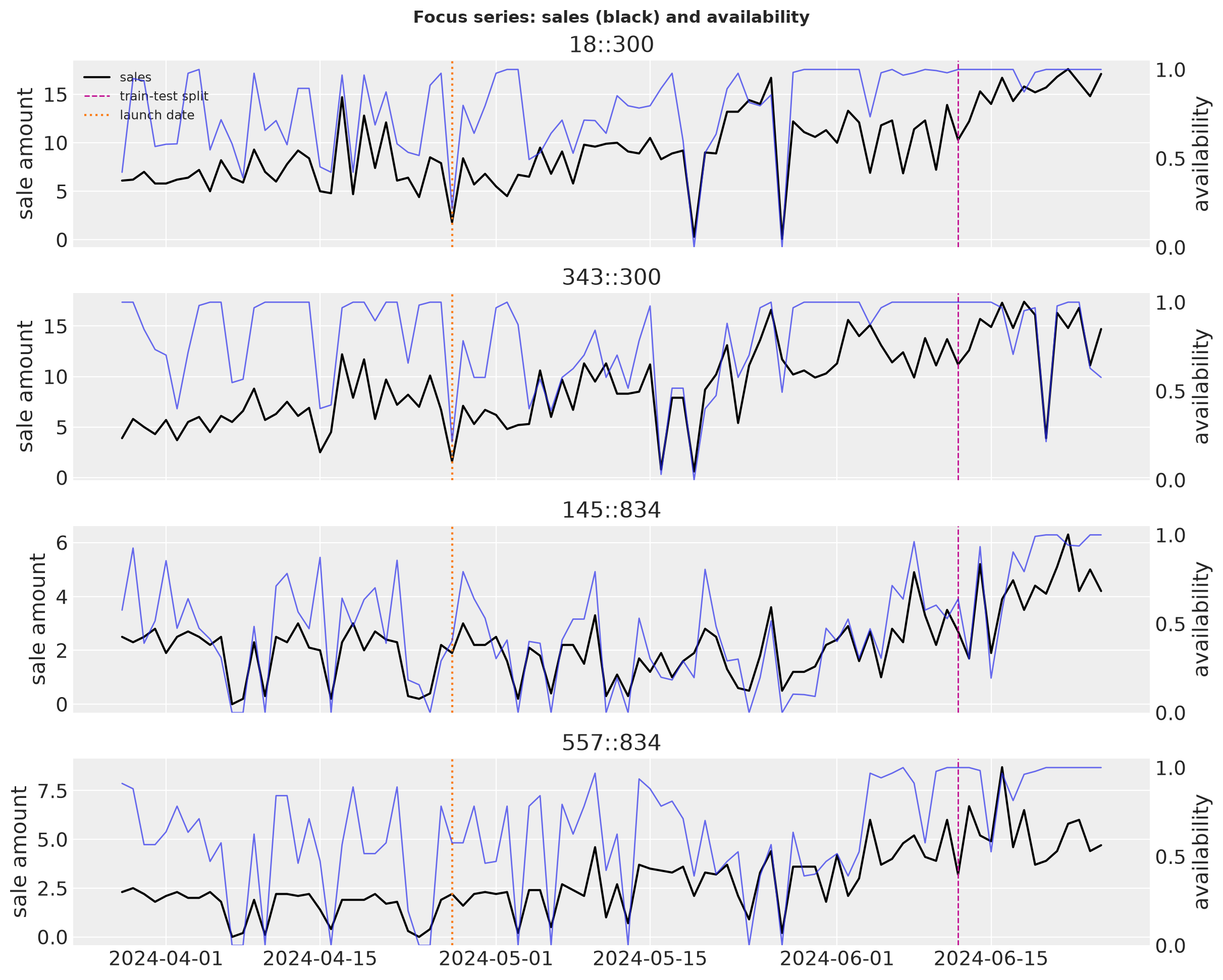
We keep the N_PER_STORE highest-selling products of the N_STORES highest-volume stores (ranked on the training window only, so no test information leaks into the panel choice) — a reduced panel with a real store hierarchy for the pooled covariate effects. Alongside availability we carry four regression features: discount magnitude (discount == 0 rows are unpriced placeholders, not free giveaways), a promotion-activity flag, a holiday flag, and a post-launch step — panel-mean sales roughly double on 2024-04-27, a platform-wide launch the upstream post identifies, and without the step covariate the random-walk levels would have to absorb it.

in_train_window = pl.col("dt").str.to_date() < (
    pl.col("dt").str.to_date().min() + pl.duration(days=T_TRAIN)
)
series_sales_lf = (
    data_lf.filter(in_train_window)
    .group_by("store_id", "product_id")
    .agg(pl.col("sale_amount").sum().alias("total_sales"))
)
top_stores_lf = (
    series_sales_lf.group_by("store_id")
    .agg(pl.col("total_sales").sum())
    .sort("total_sales", descending=True)
    .head(N_STORES)
    .select("store_id")
)
top_series_df = (
    series_sales_lf.join(top_stores_lf, on="store_id")
    .sort("total_sales", descending=True)
    .group_by("store_id", maintain_order=True)
    .head(N_PER_STORE)
    .collect(engine="streaming")
)

cleaned_discount = (
    pl.when(pl.col("discount") > 0)
    .then((1 - pl.col("discount")).clip(0.0, 1.0))
    .otherwise(0.0)
    .alias("discount_magnitude")
)
panel_df = (
    data_lf.join(
        top_series_df.lazy().select("store_id", "product_id"), on=["store_id", "product_id"]
    )
    .with_columns(
        pl.col("dt").str.to_date(),
        pl.concat_str(["store_id", "product_id"], separator="::").alias("unique_id"),
        sales_weighted_availability(hourly_weights),
        cleaned_discount,
    )
    .select(
        "dt",
        "unique_id",
        "store_id",
        "sale_amount",
        "availability",
        "discount_magnitude",
        pl.col("activity_flag").cast(pl.Float64),
        pl.col("holiday_flag").cast(pl.Float64),
    )
    .collect(engine="streaming")
    .sort("unique_id", "dt")
)

series_ids = panel_df["unique_id"].unique().sort().to_list()
dates = panel_df["dt"].unique().sort().to_numpy()


def make_pivot(value):
    """Dense (date x series) matrix of one panel column, in series_ids order."""
    pivot_df = panel_df.pivot(index="dt", on="unique_id", values=value).sort("dt")
    matrix = pivot_df.select(series_ids).to_numpy().astype(np.float64)
    if matrix.shape != (len(dates), len(series_ids)) or np.isnan(matrix).any():
        raise ValueError(f"unexpected pivot for {value!r}: shape {matrix.shape}")
    return matrix


panel_ds = xr.Dataset(
    {
        name: ((TIME_DIM, "series"), make_pivot(name))
        for name in [
            "sale_amount",
            "availability",
            "discount_magnitude",
            "activity_flag",
            "holiday_flag",
        ]
    },
    coords={TIME_DIM: dates, "series": series_ids},
)
RAMP_DATE = np.datetime64("2024-04-27")
panel_ds["post_ramp"] = (
    (panel_ds[TIME_DIM] >= RAMP_DATE).astype(np.float64).broadcast_like(panel_ds["sale_amount"])
)
print("panel:", dict(panel_ds.sizes))
print("window:", dates[0], "->", dates[-1], f"| train {T_TRAIN} days, test {HORIZON} days")

panel: {'time': 90, 'series': 200}
window: 2024-03-28 -> 2024-06-25 | train 76 days, test 14 days

Each series is scaled by its training-window mean (computed inside the train fold, so no future level leaks in): on the scaled axis 1 is an average day for every series and one set of priors fits the whole panel. Covariates are stacked into a single labeled (time, input, series) array — availability first, then the four regression features.

scale = panel_ds["sale_amount"].isel({TIME_DIM: slice(None, T_TRAIN)}).mean(TIME_DIM)
y_scaled = panel_ds["sale_amount"] / scale
y_train = y_scaled.isel({TIME_DIM: slice(None, T_TRAIN)})
y_test = panel_ds["sale_amount"].isel({TIME_DIM: slice(T_TRAIN, None)})

COVARIATE_NAMES = ["discount_magnitude", "activity_flag", "holiday_flag", "post_ramp"]
INPUT_NAMES = ["availability", *COVARIATE_NAMES]
covariates = panel_ds[INPUT_NAMES].to_dataarray(dim="input").transpose(TIME_DIM, "input", "series")
covariates_train = covariates.isel({TIME_DIM: slice(None, T_TRAIN)})

series_store = panel_df.select("unique_id", "store_id").unique().sort("unique_id")
store_ids = sorted(series_store["store_id"].unique().to_list())
store_lookup = {store: i for i, store in enumerate(store_ids)}
series_to_store = np.array([store_lookup[s] for s in series_store["store_id"].to_list()])

print(f"{len(series_ids)} series in {len(store_ids)} stores")
print(
    "sale units per scaled unit:",
    f"min {float(scale.min()):.1f} | median {float(scale.median()):.1f} | "
    f"max {float(scale.max()):.1f}",
)

200 series in 10 stores
sale units per scaled unit: min 1.7 | median 2.9 | max 8.5

total_sales = panel_ds["sale_amount"].sum(TIME_DIM)
zero_availability_days = (panel_ds["availability"] == 0.0).sum(TIME_DIM)
FOCUS_SERIES = list(
    dict.fromkeys(
        [str(s) for s in total_sales.to_series().nlargest(2).index]
        + [str(s) for s in zero_availability_days.to_series().nlargest(2).index]
    )
)

fig, axes = plt.subplots(
    len(FOCUS_SERIES), 1, figsize=(12, 2.4 * len(FOCUS_SERIES)), sharex=True, layout="constrained"
)
for ax, label in zip(axes, FOCUS_SERIES, strict=True):
    ax.plot(dates, panel_ds["sale_amount"].sel(series=label), color="black", lw=1.5, label="sales")
    ax.axvline(dates[T_TRAIN], color="C3", ls="--", lw=1, label="train-test split")
    ax.axvline(RAMP_DATE, color="C1", ls=":", lw=1.5, label="launch date")
    ax.set(title=label, ylabel="sale amount")
    ax_twin = ax.twinx()
    ax_twin.plot(dates, panel_ds["availability"].sel(series=label), color="red", lw=1, alpha=0.7)
    ax_twin.grid(False)
    ax_twin.set(ylabel="availability", ylim=(0, 1.05))
axes[0].legend(loc="upper left", fontsize=9)
fig.suptitle("Focus series: sales (black) and availability (red)", fontweight="bold")
plt.show()

The availability factor

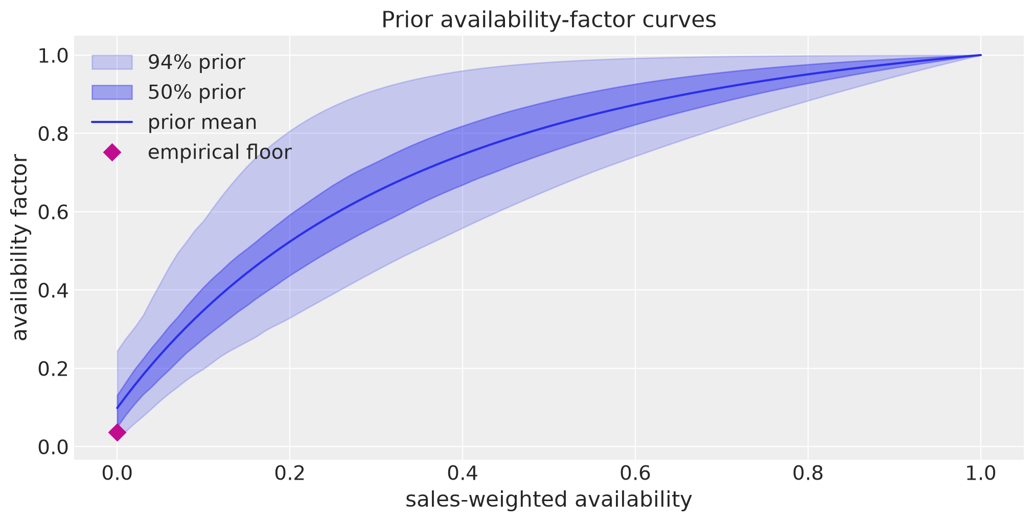
The model multiplies expected sales by a floored, saturating availability factor

$$f_{t,s} = \phi_s + (1 - \phi_s), \frac{1 - e^{-b_s, a_{t,s}}}{1 - e^{-b_s}},$$

which is exactly 1 at full availability, falls to a learned floor $\phi_s \sim \mathrm{Beta}(2, 18)$ (prior mean ≈ 0.1, covering the ~4% empirical floor) at zero availability, and bends in between with saturation rate $b_s \sim \mathrm{LogNormal}(1, 0.5)$: a large $b_s$ means a customer who wants the product almost always finds it during the hours it is in stock, so partial stockouts barely hurt. The floor is what keeps zero-availability days with positive sales from collapsing the likelihood — hard censoring (a factor of 0) would assign them zero expected sales and zero noise.

rng = np.random.default_rng(SEED)
availability_grid = np.linspace(0.0, 1.0, 101)
floor_prior = rng.beta(2.0, 18.0, size=500)
b_prior = rng.lognormal(1.0, 0.5, size=500)


def availability_factor(availability, b_avail, floor):
    """Floored, normalized saturating availability factor (NumPy version)."""
    saturation = np.expm1(-b_avail * availability) / np.expm1(-b_avail)
    return floor + (1.0 - floor) * saturation


factor_prior = availability_factor(
    availability_grid[None, :], b_prior[:, None], floor_prior[:, None]
)
quantiles = np.quantile(factor_prior, [0.03, 0.25, 0.75, 0.97], axis=0)

fig, ax = plt.subplots(figsize=(10, 5))
ax.fill_between(
    availability_grid, quantiles[0], quantiles[3], color="C0", alpha=0.2, label="94% prior"
)
ax.fill_between(
    availability_grid, quantiles[1], quantiles[2], color="C0", alpha=0.4, label="50% prior"
)
ax.plot(availability_grid, factor_prior.mean(axis=0), color="C0", label="prior mean")
ax.plot(0.0, empirical_floor, "D", color="C3", markersize=8, label="empirical floor")
ax.legend(loc="upper left")
ax.set(
    xlabel="sales-weighted availability",
    ylabel="availability factor",
    title="Prior availability-factor curves",
)
plt.show()

Model

The full generative model, per series $s$ and day $t$ on the scaled axis:

$$ \begin{aligned} \mu_{t,s} &= f_{t,s} \left( \ell_{t,s} + \gamma_{d(t),s} + \textstyle\sum_c \beta_{c,s}, x_{c,t,s} \right) \ \ell_{t,s} &= \ell_0{}{,s} + \textstyle\sum{u \le t} \sigma^{\text{drift}}s \delta{u,s} + \textstyle\sum_{u \le t} r_{u,s}, \qquad \delta_{u,s} \sim \mathrm{N}(0, 1) \ r_{t,s} &\sim \mathrm{N}(\phi^{\text{trend}}s, r{t-1,s},\ \tau^{\text{trend}}s) \qquad \text{(damped AR(1) slope)} \ \gamma{\cdot,s} &\sim \mathrm{ZeroSumNormal}(\sigma_\gamma) \quad \text{over the 7 weekdays} \ \beta_{c,s} &\sim \mathrm{N}(\mu^{\text{store}}{c,m(s)},\ \sigma^{\text{store}}{c,m(s)}) \qquad \text{(pooled by store, non-centered)} \ y_{t,s} &\sim \mathrm{N}!\left(\mu_{t,s},\ f_{t,s}\big(\sigma_s + \lambda_s,\mathrm{softplus}(\ell_{t,s})\big) + 0.02\right) \end{aligned} $$

Mapping to pymc_forecast primitives:

• the drift innovations and the slope innovations are time_series latents — in-sample steps live on "time", forecast steps on separate *_future variables the posterior never sees;

• the damped AR(1) recursion itself is a deterministic pytensor.scan over the slope innovations (the non-centered form of the AR(1)): the carry propagates from the replayed in-sample innovations straight into the forecast segment, so the horizon is conditioned through the state exactly as upstream’s Markov latent — and, unlike a random scan latent, this formulation also compiles through PyMC’s JAX log-density, which is what lets the same model run on GPU (see the fit section);

• everything carries named dims (series, store, covariate, day_of_week), so the posterior comes back fully labeled, and the weekly profile is gathered by each date’s actual calendar weekday;

• the noise scale is also multiplied by $f_{t,s}$ — stockout days have less to explain — and the constant basal term $0.02$ keeps the likelihood bounded at exact-zero sales (a learned basal scale collapses there and destabilizes the optimization);

• the upstream model learns the reparameterization centeredness with LocScaleReparam; we use plain non-centered parameterizations, the standard PyMC idiom.

DAY_NAMES = ["Mon", "Tue", "Wed", "Thu", "Fri", "Sat", "Sun"]


class FreshRetailModel(ForecastingModel):
    """Hierarchical damped-trend panel model with a floored availability factor."""

    def __init__(self, series_to_store, store_ids, covariate_names):
        super().__init__()
        self.series_to_store = series_to_store
        self.store_ids = store_ids
        self.covariate_names = covariate_names

    def model(self, h: Horizon, covariates: xr.DataArray) -> None:
        model = pm.modelcontext(None)
        model.add_coord("store", self.store_ids)
        model.add_coord("covariate", self.covariate_names)
        model.add_coord("day_of_week", DAY_NAMES)

        values = covariates.transpose(TIME_DIM, "input", "series").values
        availability = values[:, 0, :]  # (duration, series)
        features = values[:, 1:, :]  # (duration, covariate, series)
        day_index = pd.DatetimeIndex(covariates[TIME_DIM].values).dayofweek.to_numpy()

        # store-level hyperpriors for the covariate effects
        b_loc_store = pm.Normal("b_loc_store", 0.0, 0.5, dims=("covariate", "store"))
        b_scale_store = pm.HalfNormal("b_scale_store", 0.3, dims=("covariate", "store"))
        b_z = pm.Normal("b_z", 0.0, 1.0, dims=("covariate", "series"))
        b = pm.Deterministic(
            "b",
            b_loc_store[:, self.series_to_store] + b_scale_store[:, self.series_to_store] * b_z,
            dims=("covariate", "series"),
        )

        # per-series dynamics, seasonality, availability response, and noise
        drift_scale = pm.LogNormal("drift_scale", -3.0, 1.0, dims="series")
        phi_trend = pm.Beta("phi_trend", 8.0, 2.0, dims="series")
        tau_trend = pm.LogNormal("tau_trend", -4.0, 1.0, dims="series")
        init_level = pm.Normal("init_level", 1.0, 0.5, dims="series")
        seasonal_scale = pm.HalfNormal("seasonal_scale", 0.2)
        seasonal = pm.ZeroSumNormal(
            "seasonal", sigma=seasonal_scale, dims=("series", "day_of_week")
        )
        b_avail = pm.LogNormal("b_avail", 1.0, 0.5, dims="series")
        floor = pm.Beta("floor", 2.0, 18.0, dims="series")
        sigma = pm.HalfNormal("sigma", 0.5, dims="series")
        noise_loading = pm.HalfNormal("noise_loading", 0.2, dims="series")

        # random-walk drift and damped AR(1) slope over the horizon, both as
        # non-centered time_series innovations; the AR recursion is a
        # deterministic scan, so the forecast segment is conditioned through
        # the carry of the replayed in-sample innovations
        drift_z = self.time_series(
            "drift",
            lambda name, dims: pm.Normal(name, 0.0, 1.0, dims=dims),
            dims=("series",),
        )
        slope_innovation = self.time_series(
            "slope_innovation",
            lambda name, dims: pm.Normal(name, 0.0, tau_trend, dims=dims),
            dims=("series",),
        )
        slope = pytensor.scan(
            lambda innovation, previous, damping: damping * previous + innovation,
            sequences=[slope_innovation],
            outputs_info=[pt.zeros_like(init_level)],
            non_sequences=[phi_trend],
            return_updates=False,
        )

        level = init_level + pt.cumsum(drift_z * drift_scale, axis=0) + pt.cumsum(slope, axis=0)
        seasonal_rep = seasonal[:, day_index].T
        contribution = (features * b[None, :, :]).sum(axis=1)
        factor = floor + (1.0 - floor) * pt.expm1(-b_avail * availability) / pt.expm1(-b_avail)
        mu = factor * (level + seasonal_rep + contribution)
        sigma_t = factor * (sigma + noise_loading * pt.softplus(level)) + 0.02

        t_obs = h.t_obs

        def obs_fn(name, latent, dims, observed):
            noise = sigma_t[:t_obs] if dims[0] == TIME_DIM else sigma_t[t_obs:]
            return pm.Normal(name, latent, noise, dims=dims, observed=observed)

        self.predict(obs_fn, mu, dims=("series",))


model = FreshRetailModel(series_to_store, store_ids, COVARIATE_NAMES)
build_model(model, y_train, covariates_train)

\[\begin{split} \begin{array}{rcl} \text{b\_loc\_store} &\sim & \operatorname{Normal}(0,~0.5)\\\text{b\_scale\_store} &\sim & \operatorname{HalfNormal}(0,~0.3)\\\text{b\_z} &\sim & \operatorname{Normal}(0,~1)\\\text{drift\_scale} &\sim & \operatorname{LogNormal}(-3,~1)\\\text{phi\_trend} &\sim & \operatorname{Beta}(8,~2)\\\text{tau\_trend} &\sim & \operatorname{LogNormal}(-4,~1)\\\text{init\_level} &\sim & \operatorname{Normal}(1,~0.5)\\\text{seasonal\_scale} &\sim & \operatorname{HalfNormal}(0,~0.2)\\\text{seasonal} &\sim & \operatorname{ZeroSumNormal}(\text{seasonal\_scale},~\text{<constant>})\\\text{b\_avail} &\sim & \operatorname{LogNormal}(1,~0.5)\\\text{floor} &\sim & \operatorname{Beta}(2,~18)\\\text{sigma} &\sim & \operatorname{HalfNormal}(0,~0.5)\\\text{noise\_loading} &\sim & \operatorname{HalfNormal}(0,~0.2)\\\text{drift} &\sim & \operatorname{Normal}(0,~1)\\\text{slope\_innovation} &\sim & \operatorname{Normal}(0,~\text{tau\_trend})\\\text{b} &= &\operatorname{Deterministic}(f(\text{b\_z},~\text{b\_loc\_store},~\text{b\_scale\_store}))\\\text{mu} &= &\operatorname{Deterministic}(f(\text{floor},~\text{b},~\text{seasonal},~\text{init\_level},~\text{b\_avail},~\text{phi\_trend},~\text{drift},~\text{drift\_scale},~\text{slope\_innovation}))\\\text{obs} &\sim & \operatorname{Normal}(f(\text{floor},~\text{b},~\text{seasonal},~\text{init\_level},~\text{b\_avail},~\text{phi\_trend},~\text{drift},~\text{drift\_scale},~\text{slope\_innovation}),~f(\text{sigma},~\text{floor},~\text{noise\_loading},~\text{b\_avail},~\text{init\_level},~\text{phi\_trend},~\text{drift},~\text{drift\_scale},~\text{slope\_innovation})) \end{array} \end{split}\]

Inference with JAX ADVI

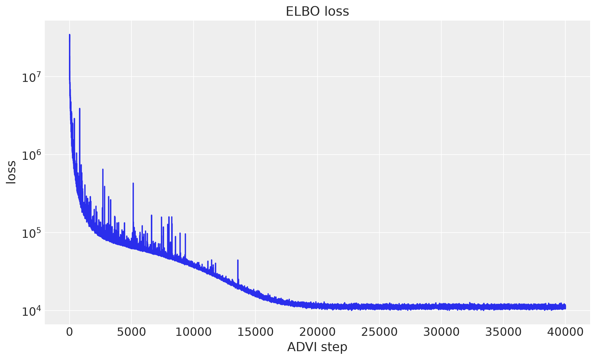
Mean-field ADVI over roughly $2 \times 76 \times 200$ time latents plus the per-series parameters. backend="jax" runs the reparameterized ELBO and Adam updates as one jax.lax.scan on the selected accelerator — the CPU here, the GPU on a machine with a CUDA JAX — while Forecaster keeps PyMC’s ordinary mean-field approximation, so posterior and predictive sampling are backend-independent. The upstream run uses a one-cycle schedule with 60k steps for the 50k-series panel; plain Adam is enough at this scale.

forecaster = Forecaster(
    model,
    y_train,
    covariates_train,
    optimizer=0.01,
    backend="jax",
    num_steps=NUM_STEPS,
    random_seed=SEED,
)

fig, ax = plt.subplots()
ax.plot(forecaster.losses)
ax.set(title="ELBO loss", xlabel="ADVI step", ylabel="loss", yscale="log")
plt.show()

Forecast

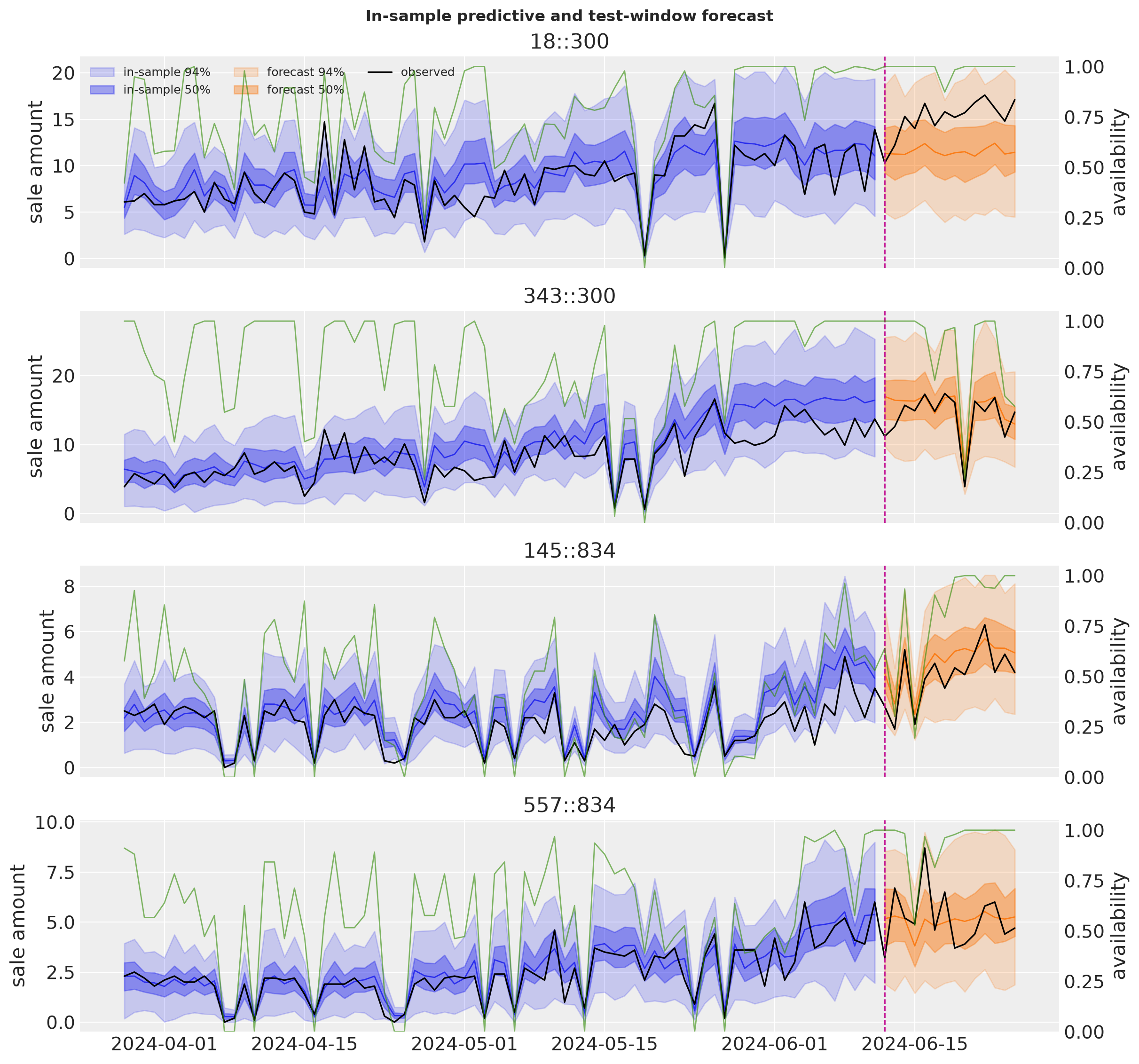
The test-window availability is known (it is observed inventory data), so the forecast conditions on it through the full-horizon covariates. We draw one posterior and reuse it for the in-sample predictive, the forecast, and the counterfactual below, so all three are conditioned on the same parameter draws.

Memory is bounded on both sides of prediction — the concern this notebook’s issue calls out (numpyro_forecast#65):

• draw_posterior(..., batch_size=...) generates the posterior in blocks and concatenates host-backed chunks. On a full-width panel the posterior draw itself is the largest avoidable allocation — the two time-by-series innovation latents alone hold draws x time x series values each.

• forecast(...) / predict_in_sample(..., batch_size=...) then replay the posterior through the predictive sampler in draw blocks as well.

At this panel size both are demonstrations; at 50,000 series they are what keeps the run from exhausting memory.

posterior = forecaster.draw_posterior(
    NUM_SAMPLES, random_seed=SEED, batch_size=POSTERIOR_BATCH_SIZE
)

pp_idata = forecaster.predict_in_sample(
    posterior=posterior, batch_size=PREDICTIVE_BATCH_SIZE, random_seed=SEED
)
fc_idata = forecaster.forecast(
    covariates, posterior=posterior, batch_size=PREDICTIVE_BATCH_SIZE, random_seed=SEED
)

# back to the original sales scale (clipped at zero: sales are non-negative)
pred_train = (pp_idata["posterior_predictive"]["obs"] * scale).clip(min=0.0)
pred_test = (fc_idata["predictions"]["forecast"] * scale).clip(min=0.0)
print("forecast dims:", dict(pred_test.sizes))

forecast dims: {'chain': 1, 'draw': 200, 'time_future': 14, 'series': 200}

Evaluation

CRPS (lower is better) and central-interval coverage on the original sales scale, against a seasonal-naive ensemble: the weekday-aligned historical windows of each series, stacked as an empirical forecast distribution — the baseline any model must beat on strongly weekly data.

def seasonal_naive_ensemble(y_history, horizon, period=7):
    """Weekday-aligned historical windows stacked as an empirical forecast ensemble."""
    t_hist = y_history.shape[0]
    windows = []
    k = 1
    while t_hist - k * period >= 0:
        start = t_hist - k * period
        if start + horizon <= t_hist:
            windows.append(y_history[start : start + horizon])
        k += 1
    return np.stack(windows)


truth_train = panel_ds["sale_amount"].isel({TIME_DIM: slice(None, T_TRAIN)})
truth_test = y_test.rename({TIME_DIM: FUTURE_DIM})
naive_test = xr.DataArray(
    seasonal_naive_ensemble(truth_train.values, HORIZON),
    dims=("draw", FUTURE_DIM, "series"),
    coords={FUTURE_DIM: truth_test[FUTURE_DIM], "series": series_ids},
)

results = pd.DataFrame(
    {
        "split": ["model (train)", "model (test)", "seasonal naive (test)"],
        "crps": [
            eval_crps(pred_train, truth_train),
            eval_crps(pred_test, truth_test),
            eval_crps(naive_test, truth_test),
        ],
        "coverage_94": [
            eval_coverage(pred_train, truth_train, alpha=0.94),
            eval_coverage(pred_test, truth_test, alpha=0.94),
            np.nan,
        ],
        "coverage_50": [
            eval_coverage(pred_train, truth_train, alpha=0.5),
            eval_coverage(pred_test, truth_test, alpha=0.5),
            np.nan,
        ],
    }
)
results.round(3)

	split	crps	coverage_94	coverage_50
0	model (train)	0.586	0.981	0.645
1	model (test)	0.844	0.922	0.516
2	seasonal naive (test)	1.131	NaN	NaN

Forecast visualization

def plot_band(ax, samples, dim, color, label):
    """Median line and 50%/94% quantile bands of a (chain, draw, time, ...) slice."""
    time_axis = samples[dim].values
    quantiles = samples.quantile([0.03, 0.25, 0.5, 0.75, 0.97], dim=("chain", "draw"))
    ax.fill_between(
        time_axis,
        quantiles.sel(quantile=0.03),
        quantiles.sel(quantile=0.97),
        color=color,
        alpha=0.2,
        label=f"{label} 94%",
    )
    ax.fill_between(
        time_axis,
        quantiles.sel(quantile=0.25),
        quantiles.sel(quantile=0.75),
        color=color,
        alpha=0.4,
        label=f"{label} 50%",
    )
    ax.plot(time_axis, quantiles.sel(quantile=0.5), color=color, lw=1)


fig, axes = plt.subplots(
    len(FOCUS_SERIES), 1, figsize=(12, 2.8 * len(FOCUS_SERIES)), sharex=True, layout="constrained"
)
for ax, label in zip(axes, FOCUS_SERIES, strict=True):
    plot_band(ax, pred_train.sel(series=label), TIME_DIM, "C0", "in-sample")
    plot_band(ax, pred_test.sel(series=label), FUTURE_DIM, "C1", "forecast")
    ax.plot(
        dates, panel_ds["sale_amount"].sel(series=label), color="black", lw=1.2, label="observed"
    )
    ax.axvline(dates[T_TRAIN], color="C3", ls="--", lw=1)
    ax.set(title=label, ylabel="sale amount")
    ax_twin = ax.twinx()
    ax_twin.plot(dates, panel_ds["availability"].sel(series=label), color="red", lw=1, alpha=0.6)
    ax_twin.grid(False)
    ax_twin.set(ylabel="availability", ylim=(0, 1.05))
axes[0].legend(loc="upper left", fontsize=9, ncols=3)
fig.suptitle("In-sample predictive and test-window forecast", fontweight="bold")
plt.show()

Demand, not sales: the counterfactual forecast

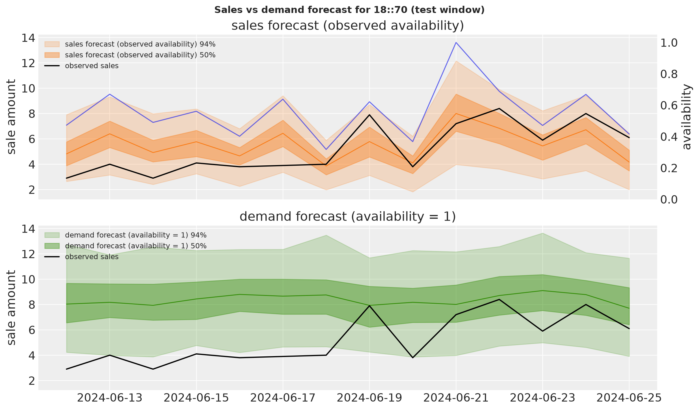
The whole point of separating demand from availability: replaying the same posterior with availability pinned to 1 over the test window forecasts what customers would buy fully in stock — the quantity to order against. On series with healthy availability the two forecasts coincide; on stockout-heavy series the demand forecast sits above the sales forecast, and the gap is the expected lost sales.

covariates_demand = covariates.copy(deep=True)
covariates_demand.loc[{"input": "availability", TIME_DIM: slice(dates[T_TRAIN], None)}] = 1.0

fc_demand_idata = forecaster.forecast(
    covariates_demand, posterior=posterior, batch_size=PREDICTIVE_BATCH_SIZE, random_seed=SEED
)
pred_test_demand = (fc_demand_idata["predictions"]["forecast"] * scale).clip(min=0.0)

demand_total = pred_test_demand.mean(("chain", "draw")).sum(FUTURE_DIM)
sales_total = pred_test.mean(("chain", "draw")).sum(FUTURE_DIM)
series_uplift = demand_total / sales_total - 1
panel_uplift = float(demand_total.sum() / sales_total.sum() - 1)
print(f"expected demand above the sales forecast on the test window: {panel_uplift:+.1%}")
print(
    f"largest per-series uplift: {float(series_uplift.max()):+.1%} "
    f"(series {series_uplift.idxmax().values!s})"
)

expected demand above the sales forecast on the test window: +9.6%
largest per-series uplift: +50.0% (series 18::70)

comparison_id = str(series_uplift.idxmax().values)
test_dates = dates[T_TRAIN:]

fig, axes = plt.subplots(2, 1, figsize=(12, 7), sharex=True, sharey=True, layout="constrained")
for ax, pred, color, label in (
    (axes[0], pred_test, "C1", "sales forecast (observed availability)"),
    (axes[1], pred_test_demand, "C2", "demand forecast (availability = 1)"),
):
    plot_band(ax, pred.sel(series=comparison_id), FUTURE_DIM, color, label)
    ax.plot(
        test_dates, y_test.sel(series=comparison_id), color="black", lw=1.5, label="observed sales"
    )
    ax.set(title=label, ylabel="sale amount")
    ax.legend(loc="upper left", fontsize=9)
ax_twin = axes[0].twinx()
ax_twin.plot(
    test_dates,
    panel_ds["availability"].isel({TIME_DIM: slice(T_TRAIN, None)}).sel(series=comparison_id),
    color="red",
    lw=1.2,
    alpha=0.7,
)
ax_twin.grid(False)
ax_twin.set(ylabel="availability", ylim=(0, 1.05))
fig.suptitle(f"Sales vs demand forecast for {comparison_id} (test window)", fontweight="bold")
plt.show()

Did the model learn the availability curve?

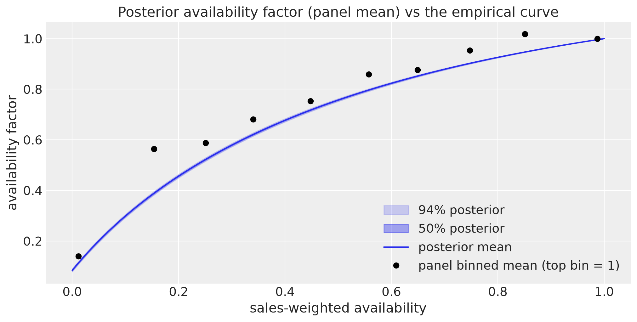
Push the posterior floor and b_avail draws through the factor formula and compare the panel-mean posterior curve with the empirical binned curve from the EDA (rescaled so its full-availability bin is 1, matching the factor’s normalization).

post = posterior[["floor", "b_avail"]].stack(sample=("chain", "draw"))
factor_draws = availability_factor(
    availability_grid[None, None, :],
    post["b_avail"].values.T[:, :, None],
    post["floor"].values.T[:, :, None],
)  # (sample, series, grid)
factor_panel = factor_draws.mean(axis=1)
post_quantiles = np.quantile(factor_panel, [0.03, 0.25, 0.75, 0.97], axis=0)

train_availability = panel_ds["availability"].isel({TIME_DIM: slice(None, T_TRAIN)})
train_scaled = y_scaled.isel({TIME_DIM: slice(None, T_TRAIN)})
bins = (train_availability * 10).astype(int).clip(0, 9).rename("availability_bin")
bin_availability = train_availability.groupby(bins).mean(...)
bin_sales = train_scaled.groupby(bins).mean(...)
top_bin = float(bin_sales.isel(availability_bin=-1))

fig, ax = plt.subplots(figsize=(10, 5))
ax.fill_between(
    availability_grid,
    post_quantiles[0],
    post_quantiles[3],
    color="C0",
    alpha=0.2,
    label="94% posterior",
)
ax.fill_between(
    availability_grid,
    post_quantiles[1],
    post_quantiles[2],
    color="C0",
    alpha=0.4,
    label="50% posterior",
)
ax.plot(availability_grid, factor_panel.mean(axis=0), color="C0", label="posterior mean")
ax.plot(
    bin_availability,
    bin_sales / top_bin,
    "o",
    color="black",
    label="panel binned mean (top bin = 1)",
)
ax.legend(loc="lower right")
ax.set(
    xlabel="sales-weighted availability",
    ylabel="availability factor",
    title="Posterior availability factor (panel mean) vs the empirical curve",
)
plt.show()

The store hierarchy at work

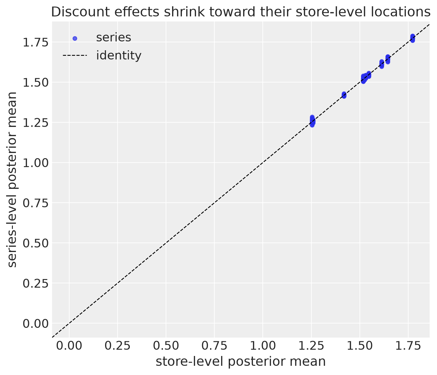
Because everything is labeled, inspecting the pooling is a sel away: each series’ discount effect shrinks toward its store’s location.

b_series = posterior["b"].sel(covariate="discount_magnitude").mean(("chain", "draw"))
b_store = posterior["b_loc_store"].sel(covariate="discount_magnitude").mean(("chain", "draw"))
b_store_per_series = b_store.values[series_to_store]

fig, ax = plt.subplots(figsize=(7, 6))
ax.scatter(b_store_per_series, b_series.values, color="C0", alpha=0.7, s=20, label="series")
ax.axline((0.0, 0.0), slope=1.0, color="black", ls="--", lw=1, label="identity")
ax.legend(loc="upper left")
ax.set(
    xlabel="store-level posterior mean",
    ylabel="series-level posterior mean",
    title="Discount effects shrink toward their store-level locations",
)
plt.show()

Scaling to the full panel

This notebook fits a few hundred series so it runs anywhere. The upstream example fits all 50,000 series on a GPU — and the code above is written to scale to that run:

• Inference on GPU. The fit already uses backend="jax", which optimizes PyMC’s mean-field ADVI objective as one jax.lax.scan on whatever accelerator JAX sees — the CPU here, a GPU wherever a CUDA JAX is installed:

  uv sync --all-extras --group notebooks
  uv pip install --upgrade "jax[cuda12]"
  

  The model body compiles through PyMC’s JAX log-density because the damped slope is a deterministic scan over time_series innovations rather than a random scan latent.

• Memory — the reason both batch_size knobs exist. At 50k series a single pass materializes draws x time x series arrays per variable (500 draws x 90 days x 50k series is ~18 GB in float64). draw_posterior(..., batch_size=50) bounds the posterior draw itself; forecast(..., batch_size=50) bounds the predictive replay (together the port of numpyro_forecast#65, where the unbatched GPU run OOMs); var_names=["forecast"] drops the *_future latents and mu_future from the output when only the forecast itself is needed.

• Data. The polars pipeline above already streams the full 4.5M-row parquet; only the panel selection constants change.

References

• Juan Orduz, Forecasting Retail Demand Under Stockouts — the upstream NumPyro version of this notebook, fit to the full 50k-series panel on GPU.

• FreshRetailNet-50K (Dingdong-Inc), CC-BY-4.0.

• pymc-forecast#47 — the issue tracking this port; numpyro_forecast#65 — the upstream batched-prediction change ported as batch_size.