M5 forecasting: top-down, bottom-up and middle-out#
This notebook ports the three models of the Pyro M5 starter kit,
as already ported to numpyro_forecast,
onto the PyMC forecasting classes. The competition panel is 30,490 daily unit-sales
series of Walmart items (3,049 items in 10 stores of 3 states), a 28-day horizon, and
42,840 aggregates across 12 hierarchy levels. The hierarchy, the covariates, the three
models, and the competition scores are defined below, next to their formulas;
load_m5 only reads the competition files.
The three models are three reconciliation strategies for the same hierarchy:
Top-down. One Student-T regression on the log of total daily sales, with a trend, weekday effects, and day-of-month effects. The forecast is exponentiated and split to the items by their share of the last 28 training days, then Poisson-sampled.
Bottom-up. A Gamma regression for every series. Mean and scale weights are shared by the items of a department in a store: three lagged log moving averages, a SNAP flag, and a weekday effect, passed through a bounded exponential. Forecasts are already at the bottom of the hierarchy and are summed up.
Middle-out. A Student-T regression on the store-by-department series, each divided by its lag-1 scale, with a trend, weekday effects, and 52 yearly Fourier harmonics. Forecasts are clipped at zero, restored to units, split to the items of each store-department, and summed up to the levels above.
Priors and formulas follow the kit. The deviations from the kit and from the numpyro_forecast port are deliberate and listed here:
Inference is mean-field ADVI through
Forecaster(Adam at the default learning rate, the JAX backend), not the kit’s clipped, decaying, minibatch SVI. Posterior draws, and therefore scores, are not expected to match a NumPyro run.The fits use a subset of the panel: the three best sellers of every department, in two California stores, one Texas store and one Wisconsin store (84 series). Every one of the 12 levels is a different set of series on this subset, so each reconciliation step does real work: the top-down split covers 84 items, the middle-out split covers 28 store-departments of 3 items each, and the bottom-up weights are shared by 3 items per store-department. The official-weight check still runs on the full panel.
The middle-out scale of a store-department is computed once on the full training window and reused in the backtest, as the kit does (numpyro_forecast rescales per window).
CI sets
PYMC_FORECAST_SMOKE_TEST=1and reruns this notebook on a synthetic three-store panel with 40 ADVI steps. That run does not download the competition files; its scores are a smoke check, not a forecast.
Prepare notebook#
Day 0 is 2011-01-29. The training file has 1,941 days; the evaluation file adds
the 28-day horizon. The bottom-up likelihood starts at day T0 = 121
(37 + 28 * 3), which is the kit’s cut, not the first day the three moving
averages are defined (that is day 111). Earlier days stay in the moving-average
history and out of the likelihood.
GAMMA_FLOOR (1e-3) clamps a Gamma mean, an incomplete moving average, and a
non-positive total before the log. The bounded exponential caps at 1e3, so an
early ADVI step cannot overflow. Poisson rates are clipped at 1e9.
import logging
import os
from functools import partial
from time import perf_counter

import arviz as az
import matplotlib.pyplot as plt
import numpy as np
import pandas as pd
import pymc as pm
import pytensor.tensor as pt
import scipy.sparse as sp
import xarray as xr

from pymc_forecast import (
    FORECAST_VAR,
    FUTURE_DIM,
    TIME_DIM,
    Forecaster,
    ForecastingModel,
    backtest,
    crps_empirical,
    fourier_features,
    prediction_samples,
    results_to_dataframe,
)
from pymc_forecast.datasets import M5Data, load_m5

logging.getLogger("pymc").setLevel(logging.ERROR)
logging.getLogger("pytensor").setLevel(logging.ERROR)
HDI_PROB = 0.94

az.style.use("arviz-darkgrid")
az.rcParams["stats.ci_kind"] = "hdi"
az.rcParams["stats.ci_prob"] = HDI_PROB
plt.rcParams["figure.figsize"] = [10, 6]
plt.rcParams["figure.dpi"] = 100
plt.rcParams["figure.facecolor"] = "white"

%config InlineBackend.figure_format = "retina"

# Twelve levels, in competition order. A bottom series belongs to one group at each.
LEVELS = {
    "Level1": (),
    "Level2": ("state_id",),
    "Level3": ("store_id",),
    "Level4": ("cat_id",),
    "Level5": ("dept_id",),
    "Level6": ("state_id", "cat_id"),
    "Level7": ("state_id", "dept_id"),
    "Level8": ("store_id", "cat_id"),
    "Level9": ("store_id", "dept_id"),
    "Level10": ("item_id",),
    "Level11": ("state_id", "item_id"),
    "Level12": ("item_id", "store_id"),
}
# Median, plus both ends of the 50%, 67%, 95%, and 99% central intervals.
M5_INTERVALS = np.array([0.5, 0.67, 0.95, 0.99])
M5_QUANTILES = np.sort(
    np.concatenate([[0.5], (1.0 - M5_INTERVALS) / 2.0, (1.0 + M5_INTERVALS) / 2.0])
)

T0 = 121
HORIZON = 28
N_DAYS_TRAIN = 1941
N_DAYS = N_DAYS_TRAIN + HORIZON
SHARE_WINDOW = 28
GAMMA_FLOOR = 1e-3
RATE_CAP = 1e9
BEXP_BOUND = 1e3
MA_WINDOWS = (28, 56, 84)
MA_LAG = 28
BOTTOM_CHANNELS = ("dow", "snap", "saled", "ma28", "ma56", "ma84")
WEEKDAYS = ("Mon", "Tue", "Wed", "Thu", "Fri", "Sat", "Sun")
HEADS = ("mean", "scale")
LAGS = ("ma28", "ma56", "ma84")
SNAP_BY_STATE = {"CA": "snap_CA", "TX": "snap_TX", "WI": "snap_WI"}
N_BACKTEST = 3  # backtest windows before the holdout, STRIDE days apart (the kit's three)
STRIDE = 35
PLOT_WEEKS = 16  # training weeks shown before the holdout in every forecast plot

SMOKE = os.environ.get("PYMC_FORECAST_SMOKE_TEST", "0") == "1"
SEED = 2026
BACKEND = "jax"
STORES = ["CA_1", "CA_2", "TX_1"] if SMOKE else ["CA_1", "CA_2", "TX_1", "WI_1"]
ITEMS_PER_DEPT = 2 if SMOKE else 3
# Smoke mode holds out the 28 days after the shortest history that still gives the
# bottom-up likelihood (from T0) room for N_BACKTEST backtest windows and a holdout.
ORIGIN = (T0 + 2 * HORIZON + (N_BACKTEST - 1) * STRIDE) if SMOKE else N_DAYS_TRAIN
STEPS = (
    {"top-down": 40, "bottom-up": 40, "middle-out": 40}
    if SMOKE
    else {"top-down": 30_000, "bottom-up": 80_000, "middle-out": 20_000}
)
SAMPLES = 20 if SMOKE else 200
print(
    "Execution mode:",
    "CI smoke check; do not interpret fit quality" if SMOKE else "example panel",
)
print(f"stores={STORES}, items per department={ITEMS_PER_DEPT}, origin={ORIGIN}")
print(f"steps={STEPS}, samples={SAMPLES}, backend={BACKEND}")
Execution mode: example panel
stores=['CA_1', 'CA_2', 'TX_1', 'WI_1'], items per department=3, origin=1941
steps={'top-down': 30000, 'bottom-up': 80000, 'middle-out': 20000}, samples=200, backend=jax
The competition panel#
load_m5 downloads Nixtla’s pinned mirror of the competition files once (a 50 MB
archive, checked against its digest) into pooch.os_cache("pymc_forecast") / "m5"
(~/.cache/pymc_forecast/m5 on Linux, ~/Library/Caches/pymc_forecast/m5 on
macOS) and reads them. sales and price come back as labeled (time, series)
panels: the series coordinate is the item-store id in sales_train_evaluation.csv
order, the time coordinate is the calendar date. The 28 evaluation days are
aligned onto the training rows from the test file, and the weekly shelf prices are
repeated across the days of their wm_yr_wk. A missing price is a missing
listing, not a zero price: the weight formula treats it as no dollar sales, and
the bottom-up saled channel treats it as a closed day.
The smoke path builds a tiny panel with the same identifier columns. It never touches the competition files.
def synthetic_m5(n_days, stores, items_per_dept):
    """Tiny hierarchy-preserving panel for the CI smoke path. No download."""
    rng = np.random.default_rng(SEED)
    departments = (
        ("FOODS_1", "FOODS"),
        ("FOODS_2", "FOODS"),
        ("FOODS_3", "FOODS"),
        ("HOBBIES_1", "HOBBIES"),
        ("HOBBIES_2", "HOBBIES"),
        ("HOUSEHOLD_1", "HOUSEHOLD"),
        ("HOUSEHOLD_2", "HOUSEHOLD"),
    )
    rows = []
    for dept, cat in departments:
        for k in range(1, items_per_dept + 1):
            item = f"{dept}_{k:03d}"
            for store in stores:
                rows.append(
                    {
                        "id": f"{item}_{store}",
                        "item_id": item,
                        "dept_id": dept,
                        "cat_id": cat,
                        "store_id": store,
                        "state_id": store.split("_", 1)[0],
                    }
                )
    keys = pd.DataFrame(rows)
    dates = pd.date_range("2011-01-29", periods=n_days, freq="D")
    coords = {TIME_DIM: dates.to_numpy(), "series": keys["id"].to_numpy()}
    sales = rng.poisson(2, size=(n_days, len(keys))).astype(np.float32)
    price = np.full((n_days, len(keys)), 1.5, dtype=np.float32)
    day = np.arange(n_days)
    calendar = pd.DataFrame(
        {
            "date": dates,
            "snap_CA": (day % 14 < 7).astype(np.float64),
            "snap_TX": (day % 14 >= 7).astype(np.float64),
            "snap_WI": np.zeros(n_days, dtype=np.float64),
        }
    )
    return M5Data(
        xr.DataArray(sales, dims=(TIME_DIM, "series"), coords=coords, name="sales"),
        xr.DataArray(price, dims=(TIME_DIM, "series"), coords=coords, name="price"),
        keys,
        calendar,
        pd.DataFrame(),
    )


if SMOKE:
    m5 = synthetic_m5(ORIGIN + HORIZON, STORES, ITEMS_PER_DEPT)
    print(f"synthetic smoke panel {dict(m5.sales.sizes)}; competition files not loaded")
else:
    m5 = load_m5()
    print(
        f"sales {dict(m5.sales.sizes)}, price {dict(m5.price.sizes)}, "
        f"calendar {len(m5.calendar)} days, weights {len(m5.weights)} rows"
    )
    assert m5.sales.sizes == {TIME_DIM: N_DAYS, "series": 30_490}
    assert m5.price.sizes == m5.sales.sizes
    assert not np.isnan(m5.sales.values).any()
m5.keys.head(3)
sales {'time': 1969, 'series': 30490}, price {'time': 1969, 'series': 30490}, calendar 1969 days, weights 42840 rows
| id | item_id | dept_id | cat_id | store_id | state_id | |
|---|---|---|---|---|---|---|
| 0 | HOBBIES_1_001_CA_1 | HOBBIES_1_001 | HOBBIES_1 | HOBBIES | CA_1 | CA |
| 1 | HOBBIES_1_002_CA_1 | HOBBIES_1_002 | HOBBIES_1 | HOBBIES | CA_1 | CA |
| 2 | HOBBIES_1_003_CA_1 | HOBBIES_1_003 | HOBBIES_1 | HOBBIES | CA_1 | CA |
Twelve levels#
Each aggregate is a sum of bottom series. Level 1 is the total. Levels 2–5 are state, store, category, and department. Levels 6–9 cross those. Levels 10–12 are the item, the item in a state, and the item in a store — level 12 is the bottom series itself.
A bottom series belongs to exactly one group at each level. The group id is the
rank of the sorted Agg_Level_1/Agg_Level_2 label, which is also the key in
weights_evaluation.csv once the level name is prefixed. Sorting is part of the
contract: an unsorted id would still sum the right series, and then fail the
official-weight join.
The full panel is 30,490 series by 42,840 aggregates. A dense matrix would be about 10 GB, and each series contributes exactly twelve ones, so the sum is a CSR matrix with one row per bottom series and one column per aggregate.
class Aggregation:
    """Sparse sum from bottom series to the twelve levels.

    ``group_index[level]`` maps each bottom series to a column of that level,
    in sorted label order. ``labels`` are ``Level/Agg_Level_1/Agg_Level_2``.
    """

    def __init__(self, matrix, labels, slices, group_index):
        self.matrix = matrix
        self.labels = labels
        self.slices = slices
        self.group_index = group_index

    def labels_for(self, level):
        """``Agg_Level_1/Agg_Level_2`` labels of one level, sorted."""
        sl = self.slices[level]
        return [label.split("/", 1)[1] for label in self.labels[sl]]

    def sizes(self):
        """Number of aggregates per level, in competition order."""
        return {level: sl.stop - sl.start for level, sl in self.slices.items()}

    def members(self, level):
        """The set of bottom-series sets that make up one level."""
        columns = self.matrix.tocsc()
        sl = self.slices[level]
        return frozenset(
            frozenset(columns.indices[columns.indptr[j] : columns.indptr[j + 1]].tolist())
            for j in range(sl.start, sl.stop)
        )


def _pair_label(keys, columns):
    if not columns:
        return pd.Series(["Total/X"] * len(keys), index=keys.index)
    first = keys[columns[0]].astype(str)
    second = pd.Series("X", index=keys.index) if len(columns) == 1 else keys[columns[1]].astype(str)
    return first + "/" + second


def build_aggregation(keys):
    """Hierarchy of ``keys``. Group ids follow sorted label order."""
    missing = [
        column for columns in LEVELS.values() for column in columns if column not in keys.columns
    ]
    if missing:
        raise ValueError(f"keys are missing {sorted(set(missing))}")
    n_series = len(keys)
    rows, cols, labels = [], [], []
    slices, group_index = {}, {}
    offset = 0
    for level, columns in LEVELS.items():
        pairs = _pair_label(keys, columns)
        ordered = sorted(pairs.unique())
        index = {label: i for i, label in enumerate(ordered)}
        groups = pairs.map(index).to_numpy(dtype=np.int64)
        group_index[level] = groups
        rows.append(np.arange(n_series))
        cols.append(offset + groups)
        labels.extend(f"{level}/{label}" for label in ordered)
        slices[level] = slice(offset, offset + len(ordered))
        offset += len(ordered)
    matrix = sp.csr_matrix(
        (
            np.ones(n_series * len(LEVELS), dtype=np.float64),
            (np.concatenate(rows), np.concatenate(cols)),
        ),
        shape=(n_series, offset),
    )
    return Aggregation(matrix, labels, slices, group_index)


def aggregate(values, matrix):
    """Sum the last axis through a ``(n_series, n_aggregates)`` matrix."""
    values = np.asarray(values, dtype=np.float64)
    if values.shape[-1] != matrix.shape[0]:
        raise ValueError(
            f"last axis is {values.shape[-1]}, aggregation expects {matrix.shape[0]} series"
        )
    flat = values.reshape(-1, matrix.shape[0])
    summed = matrix.T.dot(flat.T).T
    return summed.reshape(*values.shape[:-1], matrix.shape[1])


def log_total(sales, *, floor=GAMMA_FLOOR):
    """Log of the panel total. Non-positive totals are floored first."""
    total = np.asarray(sales, dtype=np.float64).sum(-1)
    return np.log(np.maximum(total, floor))


def level_panel(sales, aggregation, level):
    """One level's columns, in the matrix's sorted-label order."""
    sl = aggregation.slices[level]
    return aggregate(sales, aggregation.matrix)[..., sl]


def level_table(aggregation):
    """Level, grouping, and number of aggregates, one row per level."""
    return pd.DataFrame(
        [
            {
                "level": level,
                "grouping": " x ".join(columns) if columns else "total",
                "series": size,
            }
            for (level, columns), size in zip(
                LEVELS.items(), aggregation.sizes().values(), strict=True
            )
        ]
    )
Covariates#
Weekday is Monday = 0, taken from the calendar date. years is the row number
divided by 365, matching the kit rather than a 365.25 year. Christmas is
December 25. SNAP is the flag of the series’ own state.
The top-down design is years, weekday, and 31 day-of-month dummies. The
middle-out design replaces the dummies with 52 yearly Fourier harmonics at period
365.25, a sine and a cosine each (sin_1 … cos_52, 104 columns), from
fourier_features. Both are built on the day prefix that ends at the holdout and
starts at day 0, so the trend and the Fourier phase match the kit’s calendar.
The bottom-up design has six channels, one value per series per day:
dow, the shared weekday, broadcast to every series;snap, the state SNAP flag;saled, 1 when a price is listed and the day is not Christmas, else 0;ma28,ma56,ma84: the log of the mean sales over that window, ending 28 days before the current day.
A moving average without a full window is log(1e-3). The averages are
computed on sales before the later T0 slice, so a likelihood that starts
at day 121 still sees the earlier history. The 28-day lag means the holdout
does not enter them: at forecast time the future averages are known.
def calendar_features(calendar):
    """Weekday, years-since-start, Christmas, day-of-month dummies, SNAP flags."""
    if "date" not in calendar.columns:
        raise ValueError("calendar is missing date")
    dates = pd.to_datetime(calendar["date"])
    out = pd.DataFrame(
        {
            "dow": dates.dt.dayofweek.to_numpy(dtype=np.int64),
            "years": np.arange(len(dates), dtype=np.float64) / 365.0,
            "christmas": ((dates.dt.month == 12) & (dates.dt.day == 25)).to_numpy(dtype=np.float64),
        }
    )
    for day in range(1, 32):
        out[f"dom_{day}"] = (dates.dt.day == day).to_numpy(dtype=np.float64)
    missing = [column for column in SNAP_BY_STATE.values() if column not in calendar.columns]
    if missing:
        raise ValueError(f"calendar is missing {missing}")
    for column in SNAP_BY_STATE.values():
        out[column] = calendar[column].to_numpy(dtype=np.float64)
    return out


def _time_index(calendar, n_days):
    if len(calendar) != n_days:
        raise ValueError(f"calendar has {len(calendar)} rows, expected {n_days}")
    dates = pd.to_datetime(calendar["date"])
    if dates.duplicated().any():
        raise ValueError("calendar dates are not unique")
    return dates.to_numpy()


def top_covariates(calendar):
    """Years, weekday, and 31 day-of-month dummies."""
    features = calendar_features(calendar)
    columns = ["years", "dow", *[f"dom_{day}" for day in range(1, 32)]]
    return xr.DataArray(
        features[columns].to_numpy(dtype=np.float64),
        dims=(TIME_DIM, "feature"),
        coords={TIME_DIM: _time_index(calendar, len(features)), "feature": columns},
        name="covariates",
    )


def middle_covariates(calendar):
    """Years, weekday, and 52 yearly Fourier pairs."""
    features = calendar_features(calendar)
    fourier = fourier_features(len(features), period=365.25, num_terms=52)
    names = ["years", "dow", *fourier.coords["fourier"].values.tolist()]
    values = np.column_stack(
        [features["years"].to_numpy(), features["dow"].to_numpy(), fourier.values]
    )
    return xr.DataArray(
        values,
        dims=(TIME_DIM, "feature"),
        coords={TIME_DIM: _time_index(calendar, len(features)), "feature": names},
        name="covariates",
    )


def lagged_log_moving_average(y, window, lag, *, floor=GAMMA_FLOOR):
    """Log mean over ``window`` days ending ``lag`` days before each day.

    Days without a full window are ``log(floor)``. The cumulative sum is float64.
    """
    values = np.asarray(y, dtype=np.float64)
    padded = np.concatenate([np.zeros((1, values.shape[1])), np.cumsum(values, axis=0)])
    t = np.arange(values.shape[0])
    stop = np.clip(t - lag + 1, 0, None)
    start = np.clip(stop - window, 0, None)
    mean = (padded[stop] - padded[start]) / window
    mean[t - lag + 1 - window < 0] = 0.0
    return np.log(np.maximum(mean, floor))


def bottom_covariates(sales, price, calendar, keys):
    """Weekday, SNAP, listed-and-open, and three lagged log moving averages."""
    sales = np.asarray(sales, dtype=np.float64)
    price = np.asarray(price, dtype=np.float64)
    features = calendar_features(calendar)
    christmas = features["christmas"].to_numpy()
    saled = (~np.isnan(price)).astype(np.float64) * (1.0 - christmas[:, None])
    state_index = np.array(
        [list(SNAP_BY_STATE).index(state) for state in keys["state_id"].astype(str)]
    )
    snap_table = features[list(SNAP_BY_STATE.values())].to_numpy(dtype=np.float64)
    channels = {
        "dow": np.broadcast_to(features["dow"].to_numpy()[:, None], sales.shape).copy(),
        "snap": snap_table[:, state_index],
        "saled": saled,
    }
    for window, name in zip(MA_WINDOWS, LAGS, strict=True):
        channels[name] = lagged_log_moving_average(sales, window, MA_LAG)
    values = np.stack([channels[name] for name in BOTTOM_CHANNELS], axis=-1)
    return xr.DataArray(
        values,
        dims=(TIME_DIM, "series", "channel"),
        coords={
            TIME_DIM: _time_index(calendar, sales.shape[0]),
            "series": keys["id"].astype(str).to_numpy(),
            "channel": list(BOTTOM_CHANNELS),
        },
        name="covariates",
    )


def select_series(keys, sales, *, stores, items_per_dept, origin):
    """Ids of the ``items_per_dept`` best sellers of each department, in ``stores``.

    An item is ranked by its unit sales over the ``origin`` training days summed
    over the chosen stores, so the same items are kept in every store and every
    store-department holds the same number of items. Ids come back in sales-file
    order, ready for ``.sel(series=...)``.
    """
    frame = keys.reset_index(drop=True)
    in_stores = frame["store_id"].astype(str).isin(stores).to_numpy()
    totals = np.asarray(sales, dtype=np.float64)[:origin].sum(0)
    ranked = (
        frame.assign(total=np.where(in_stores, totals, 0.0))
        .groupby(["dept_id", "item_id"], sort=False)["total"]
        .sum()
        .reset_index()
        .sort_values(["dept_id", "total", "item_id"], ascending=[True, False, True])
    )
    chosen = set(ranked.groupby("dept_id", sort=False).head(items_per_dept)["item_id"])
    mask = in_stores & frame["item_id"].isin(chosen).to_numpy()
    if not mask.any():
        raise ValueError("selection is empty")
    return frame.loc[mask, "id"].astype(str).to_numpy()
Reconciliation and the competition scores#
Top-down exponentiates the log-total forecast and treats every item as a member of one group. Middle-out clips the level-9 forecast at zero, multiplies it back by the training-window scale, and splits inside each store-department. Bottom-up is already a bottom-level draw; it is not passed through this split.
The split is Poisson. The rate of a series is its group’s draw times its share
of that group’s sales over the last 28 training days. A group whose total is
zero is split uniformly. Non-finite rates are clipped to [0, 1e9]. Draws
follow the C-order ravel of the rate, in blocks only to bound the temporary, so
the seed fixes the Poisson noise and not the ADVI draws.
Scoring aggregates those bottom draws back up the same matrix. For each level, weighted scaled CRPS is the horizon-mean empirical CRPS, times the level’s weight, divided by the level’s scale, summed inside the level; the headline score is the mean over the twelve levels:
WSPL is the pinball loss at the nine competition quantiles — the median and both ends of the 50%, 67%, 95%, and 99% intervals, \(0.005, 0.025, 0.165, 0.25, 0.5, 0.75, 0.835, 0.975, 0.995\) — mean over quantiles and the horizon, weighted and scaled the same way, then averaged across the twelve levels. Lower is better. On this subset the numbers are not competition scores.
def last_28_day_shares(train_sales, group_index, *, window=SHARE_WINDOW):
    """Share of each series in its group's sales over the last ``window`` days.

    A group whose total is zero is split uniformly across its members.
    """
    sales = np.asarray(train_sales, dtype=np.float64)
    groups = np.asarray(group_index, dtype=np.int64)
    totals = sales[-window:].sum(0)
    n_groups = int(groups.max()) + 1 if groups.size else 0
    group_totals = np.bincount(groups, weights=totals, minlength=n_groups)
    group_sizes = np.bincount(groups, minlength=n_groups)
    positive = group_totals[groups] > 0.0
    shares = np.empty(groups.shape, dtype=np.float64)
    shares[positive] = totals[positive] / group_totals[groups][positive]
    shares[~positive] = 1.0 / group_sizes[groups][~positive]
    return shares


def disaggregate(seed, group_draws, shares, group_index, *, chunk=50, rate_cap=RATE_CAP):
    """Poisson bottom draws with rate ``group draw * share``.

    The chunk only bounds the temporary. Draws follow the C-order ravel, so a
    different chunk does not change the seeded result.
    """
    draws = np.asarray(group_draws)
    share = np.asarray(shares, dtype=np.float64)
    groups = np.asarray(group_index, dtype=np.int64)
    rate = np.asarray(draws[..., groups], dtype=np.float64) * share
    rate = np.clip(np.nan_to_num(rate, nan=0.0, posinf=rate_cap, neginf=0.0), 0.0, rate_cap)
    flat = np.ascontiguousarray(rate).ravel()
    rng = np.random.default_rng(seed)
    out = np.empty(flat.shape, dtype=np.float32)
    trailing = int(np.prod(rate.shape[1:], dtype=int)) if rate.ndim > 1 else flat.size or 1
    block = max(int(chunk), 1) * trailing
    cursor = 0
    while cursor < flat.size:
        stop = min(cursor + block, flat.size)
        out[cursor:stop] = rng.poisson(flat[cursor:stop])
        cursor = stop
    return out.reshape(rate.shape)


def forecast_draws(result):
    """Forecast samples as ``(sample, horizon, series)``, from a prediction tree or array."""
    samples = result if isinstance(result, xr.DataArray) else prediction_samples(result)["forecast"]
    if "chain" in samples.dims and "draw" in samples.dims:
        samples = samples.stack(sample=("chain", "draw"))
    elif "draw" in samples.dims:
        samples = samples.rename(draw="sample")
    time_dim = FUTURE_DIM if FUTURE_DIM in samples.dims else TIME_DIM
    others = [dim for dim in samples.dims if dim not in ("sample", time_dim)]
    return np.asarray(samples.transpose("sample", time_dim, *others).values, dtype=np.float64)


def reconcile_top_down(forecast, origin):
    """Exponentiate a log-total forecast and split it by the shares before ``origin``."""
    units = np.exp(forecast_draws(forecast))
    groups = np.zeros(panel_sales.shape[1], dtype=np.int64)
    shares = last_28_day_shares(panel_sales[:origin], groups)
    return disaggregate(SEED + origin, units, shares, groups)


def reconcile_middle_out(forecast, origin):
    """Clip a scaled level-9 forecast at zero, restore units, and split within each group."""
    units = np.clip(forecast_draws(forecast), 0.0, None) * scale_mid
    groups = panel.group_index["Level9"]
    shares = last_28_day_shares(panel_sales[:origin], groups)
    return disaggregate(SEED + origin, units, shares, groups)


def reconcile_bottom_up(forecast, origin):
    """Bottom-level draws need no split."""
    return forecast_draws(forecast)


def ws_crps_level(pred, truth, *, sl, weights, scales):
    """Weighted scaled CRPS of one level from draws and truth on all aggregates."""
    crps = crps_empirical(pred[..., sl], truth[..., sl]).mean(axis=0)
    return float(np.sum(weights * crps / scales))


def m5_window_metrics(t0, t1, t2, *, offset=0):
    """The twelve per-level WS-CRPS metrics of a window whose training ends at ``t1 + offset``.

    ``offset`` is the panel day of the first row of the series handed to ``backtest``.
    """
    origin = t1 + offset
    weights = m5_weights(panel_sales, panel_price, panel, origin)
    scales = m5_scales(aggregate(panel_sales[:origin], panel.matrix))
    return {
        f"ws_crps_{level}": partial(ws_crps_level, sl=sl, weights=weights[sl], scales=scales[sl])
        for level, sl in panel.slices.items()
    }


def ws_pinball(pred, truth, weights, scales):
    """M5 WSPL: pinball loss at the nine quantiles, weighted, scaled, mean over levels."""
    quantiles = np.quantile(pred, M5_QUANTILES, axis=0)
    error = quantiles - truth[None]
    u = M5_QUANTILES[:, None, None]
    # Pinball: u*(y-q) when the quantile is below the truth, else (1-u)*(q-y).
    per_series = (np.where(error <= 0.0, -u, 1.0 - u) * error).mean(axis=(0, 1))
    level_scores = [
        np.sum(weights[sl] * per_series[sl] / scales[sl]) for sl in panel.slices.values()
    ]
    return float(np.mean(level_scores))


def score_holdout(bottom_draws):
    """Per-level WS-CRPS and WSPL of bottom draws against the holdout after ``ORIGIN``."""
    draws = np.asarray(bottom_draws, dtype=np.float64)
    assert draws.shape[1:] == (HORIZON, panel_sales.shape[1])
    assert np.isfinite(draws).all()
    pred = aggregate(draws, panel.matrix)
    truth = aggregate(panel_sales[ORIGIN:end], panel.matrix)
    metrics = m5_window_metrics(0, ORIGIN, end)
    scores = {level: metrics[f"ws_crps_{level}"](pred, truth) for level in LEVELS}
    weights = m5_weights(panel_sales, panel_price, panel, ORIGIN)
    scales = m5_scales(aggregate(panel_sales[:ORIGIN], panel.matrix))
    return scores, ws_pinball(pred, truth, weights, scales)


def mean_level_score(scores):
    """Mean of the twelve level scores, in competition order."""
    return float(np.mean([scores[level] for level in LEVELS]))
Fit#
Each model is a ForecastingModel. One definition trains and forecasts:
predict registers the in-sample likelihood on "obs" and the horizon draw
on "forecast". Forecaster fits the training slice with mean-field ADVI (Adam
at the default learning rate; the JAX backend runs the ELBO and the updates as
one compiled scan), draw_posterior draws the parameters once, and the same
draws feed predict_in_sample and forecast, so the in-sample bands and the
forecast bands below come from the same parameter draws. The future weekday,
SNAP flag, and lagged averages are known at forecast time.
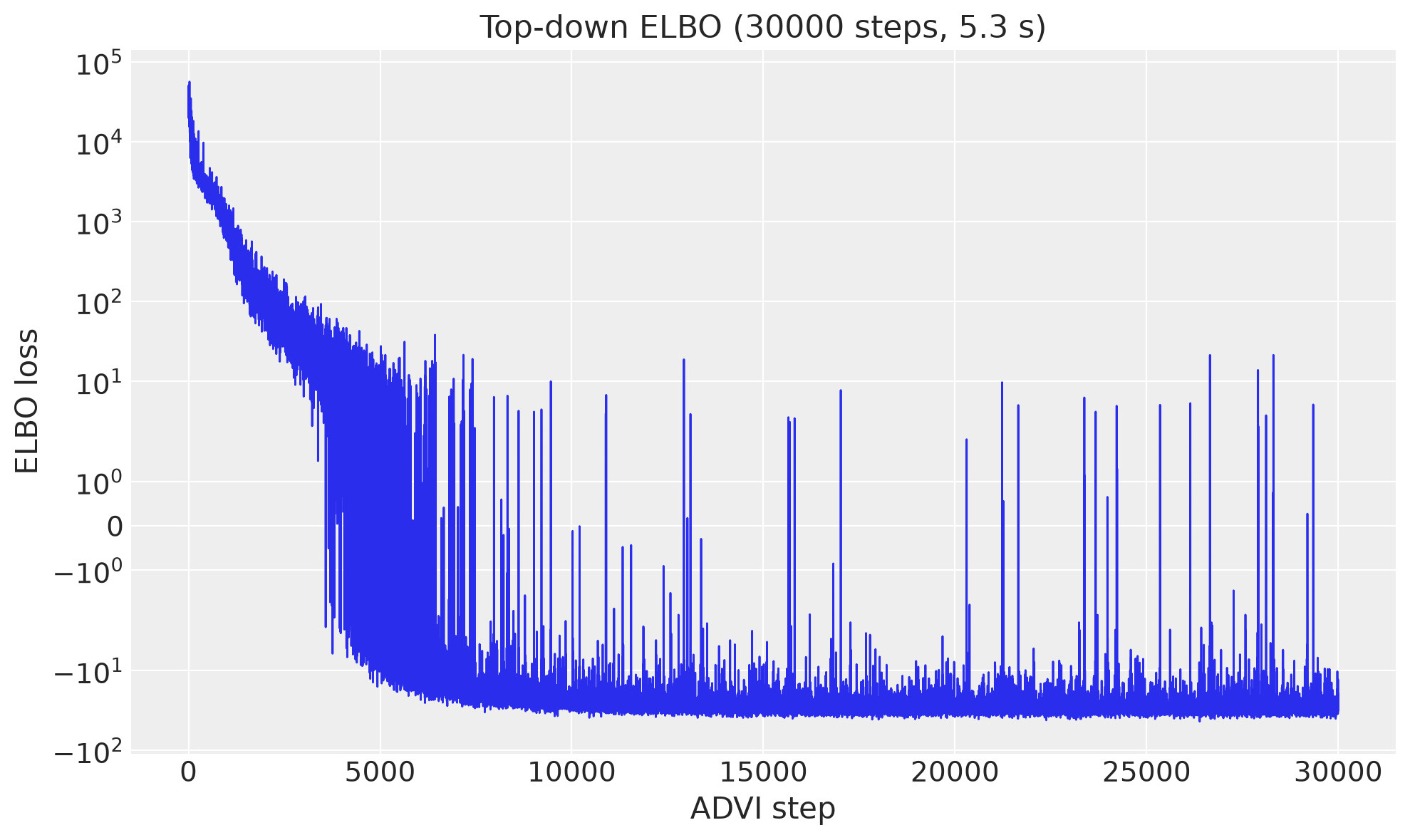
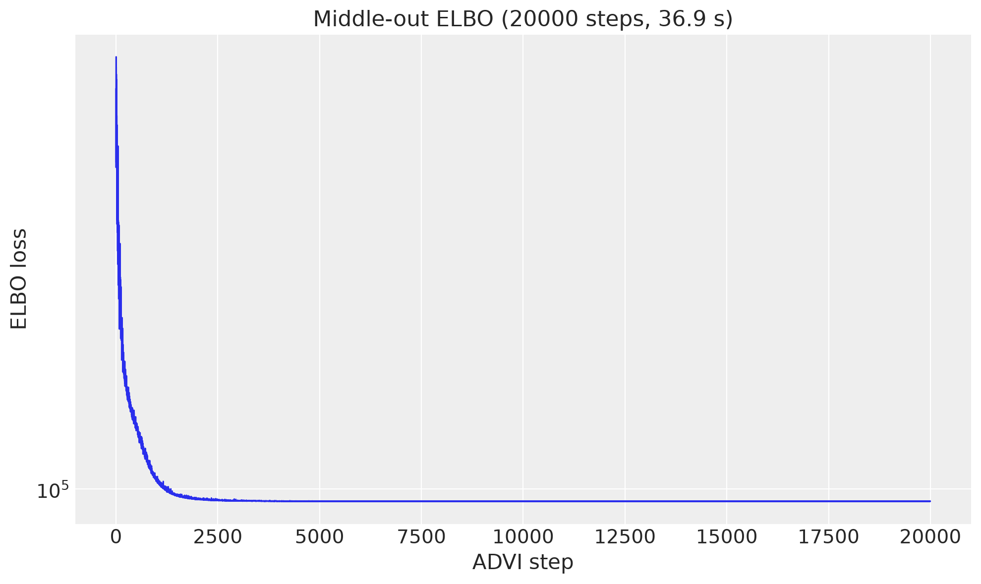
The step counts are round counts at which every fit passes the package’s ELBO check (no “still descending” warning) on this panel: 30,000 for the top-down model, 20,000 for the middle-out model, and 80,000 for the bottom-up Gamma regression, whose loss is still falling at 40,000 even with a higher learning rate. That check is a heuristic, so the backtest at the end of the notebook is the real test: three more fits of each model with their own seeds and training windows. The bottom-up fits dominate the run time, about three minutes each.
def fit_and_forecast(model, data, covariates, steps):
    """Fit on the training slice, draw the posterior once, forecast the horizon."""
    train_cov = covariates.sel({TIME_DIM: data[TIME_DIM].values})
    started = perf_counter()
    forecaster = Forecaster(
        model,
        data,
        train_cov,
        num_steps=steps,
        backend=BACKEND,
        random_seed=SEED,
        progressbar=False,
    )
    elapsed = perf_counter() - started
    posterior = forecaster.draw_posterior(SAMPLES, random_seed=SEED)
    predicted = forecaster.forecast(
        covariates, posterior=posterior, random_seed=SEED, progressbar=False
    )
    return forecaster, posterior, predicted, elapsed


def plot_loss(losses, title):
    fig, ax = plt.subplots()
    ax.plot(np.asarray(losses), color="C0", lw=1)
    ax.set_yscale("symlog")
    ax.set(title=title, xlabel="ADVI step", ylabel="ELBO loss")
    fig.tight_layout()
    plt.show()


def add_bands(ax, x, draws, *, color, label):
    """90% and 50% quantile bands and the median of ``(sample, time)`` draws."""
    q = np.quantile(draws, [0.05, 0.25, 0.5, 0.75, 0.95], axis=0)
    ax.fill_between(x, q[0], q[4], color=color, alpha=0.25, lw=0, label=f"{label} 90%")
    ax.fill_between(x, q[1], q[3], color=color, alpha=0.5, lw=0, label=f"{label} 50%")
    ax.plot(x, q[2], color=color, lw=1)


def plot_window(ax, in_sample, forecast, observed, *, title, ylabel):
    """Last training weeks in blue (in-sample), the holdout in orange (forecast), truth in black.

    ``in_sample`` is ``(sample, ORIGIN)`` or ``None``; ``forecast`` is ``(sample, HORIZON)``;
    ``observed`` covers the ``end`` days of the panel.
    """
    start = max(0, ORIGIN - 7 * PLOT_WEEKS)
    if in_sample is not None:
        add_bands(ax, time[start:ORIGIN], in_sample[:, start:ORIGIN], color="C0", label="in-sample")
    add_bands(ax, time[ORIGIN:end], forecast, color="C1", label="forecast")
    ax.plot(time[start:end], observed[start:end], color="black", lw=1, label="observed")
    ax.axvline(time[ORIGIN], color="gray", ls="--", lw=1)
    ax.set(title=title, ylabel=ylabel)


plot_start = max(0, ORIGIN - 7 * PLOT_WEEKS)
results = {}
Top-down#
One regression on the log of total daily sales. The Student-T location is
\(b \sim \mathrm{Normal}(0, 10)\), \(\tau \sim \mathrm{LogNormal}(-2, 1)\),
each day-of-month weight is \(\mathrm{Normal}(0, 1)\), the weekday effect is
\(\mathrm{Normal}(0, 5)\), the degrees of freedom are \(\mathrm{Uniform}(1, 10)\),
and the noise scale is \(\mathrm{LogNormal}(-2, 1)\). predict adds that noise
in-sample and draws the same noise on the horizon. The reconciliation above
then exponentiates and applies the Poisson split.
The intercept, the seven weekday effects and the 31 day-of-month dummies are collinear (a constant can move between them), as in the kit; the mean-field posterior picks one split, so the forest plots are to be read for their relative pattern.
class TopDownModel(ForecastingModel):
    """Trend, weekday, and day-of-month effects on the log total."""

    def model(self, covariates, data=None):
        years = np.asarray(covariates.sel(feature="years").values)
        dow = np.asarray(covariates.sel(feature="dow").values).astype(np.int32)
        dom_names = [
            str(name)
            for name in covariates.coords["feature"].values
            if str(name).startswith("dom_")
        ]
        dom = np.asarray(covariates.sel(feature=dom_names).values, dtype=np.float64)
        model = pm.modelcontext(None)
        model.add_coord("day_of_week", list(WEEKDAYS))
        model.add_coord("dom", dom_names)
        bias = pm.Normal("bias", 0.0, 10.0)
        trend = pm.LogNormal("trend", -2.0, 1.0)
        weight = pm.Normal("weight", 0.0, 1.0, dims="dom")
        seasonal = pm.Normal("seasonal", 0.0, 5.0, dims="day_of_week")
        prediction = bias + trend * years + seasonal[dow] + pt.dot(dom, weight)
        dof = pm.Uniform("dof", 1.0, 10.0)
        noise_scale = pm.LogNormal("noise_scale", -2.0, 1.0)
        # The extra axis is the single "total" series coord on y_top.
        self.predict(
            pm.StudentT.dist(nu=dof, mu=0.0, sigma=noise_scale),
            prediction[:, None],
        )
top, top_posterior, top_forecast, top_seconds = fit_and_forecast(
    TopDownModel(), y_top, cov_top, STEPS["top-down"]
)
plot_loss(top.losses, f"Top-down ELBO ({STEPS['top-down']} steps, {top_seconds:.1f} s)")
az.summary(top_posterior, var_names=["bias", "trend", "dof", "noise_scale"])
/var/folders/cm/3dzy9rdd5s3672z0s1brjkvh0000gn/T/ipykernel_69810/3881171391.py:27: UserWarning: The figure layout has changed to tight
  fig.tight_layout()
| mean | sd | hdi94_lb | hdi94_ub | ess_bulk | ess_tail | r_hat | mcse_mean | mcse_sd | |
|---|---|---|---|---|---|---|---|---|---|
| bias | 3.6711 | 0.0039 | 3.7 | 3.7 | 258 | 188 | nan | 0.00024 | 0.00021 |
| trend | 0.0039 | 0.0012 | 0.0019 | 0.0061 | 194 | 165 | nan | 8.7e-05 | 7e-05 |
| dof | 4.72 | 0.33 | 4.1 | 5.3 | 171 | 170 | nan | 0.026 | 0.017 |
| noise_scale | 0.1713 | 0.0032 | 0.17 | 0.18 | 196 | 165 | nan | 0.00023 | 0.00016 |
The total of this panel is flat over the five years (the best sellers were chosen over the whole training window), so the trend comes out at about 0.004 per year on the log scale with the positive LogNormal prior keeping it just above zero. The Student-T has about 4.7 degrees of freedom and a noise scale of 0.17 on the log scale: the total of 84 items moves a lot more from day to day than the total of 30,490 (where numpyro_forecast finds 0.08), and the heavy tails absorb the Christmas days, when the panel sells a handful of units. The forest plots show the weekday and day-of-month effects; their absolute level is the share of the intercept the mean-field posterior gave them, only the differences are meaningful.
pc = az.plot_forest(
    top_posterior, var_names=["seasonal"], combined=True, figure_kwargs={"figsize": (8, 3.5)}
)
pc.viz["figure"].item().suptitle("Top-down: weekday effects on the log total", fontsize=13)
pc = az.plot_forest(
    top_posterior, var_names=["weight"], combined=True, figure_kwargs={"figsize": (8, 8)}
)
pc.viz["figure"].item().suptitle("Top-down: day-of-month effects on the log total", fontsize=13);
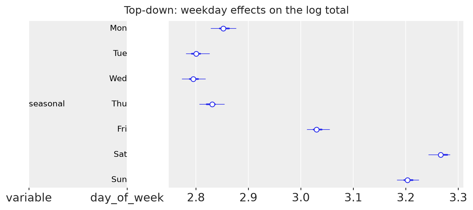
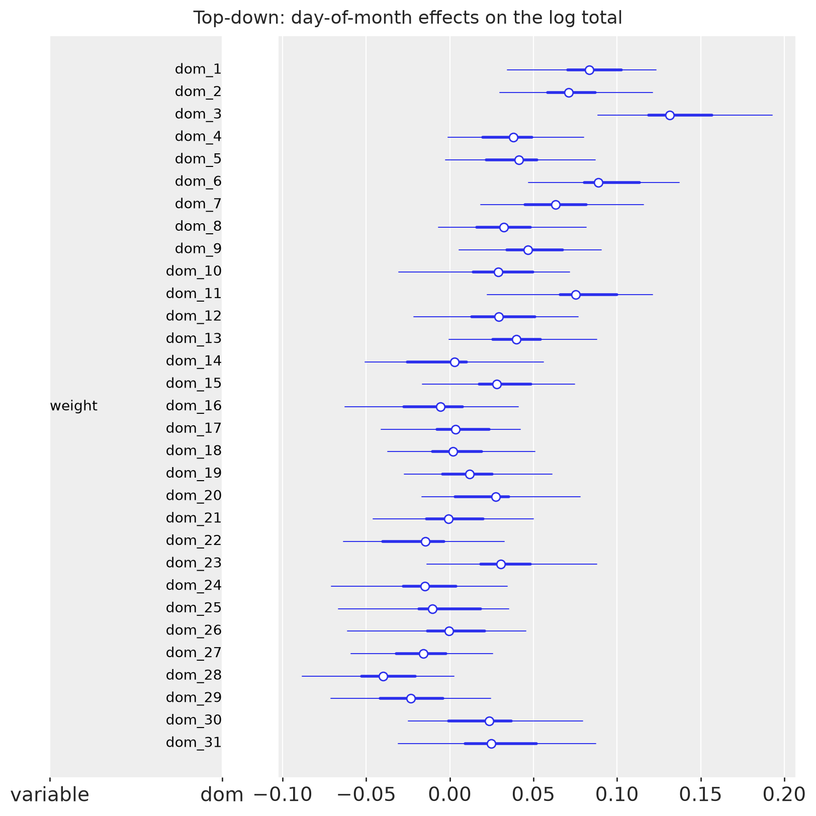
The weekend peak is about 0.45 above Tuesday and Wednesday on the log scale, some 55% more units, with Friday halfway and Sunday a little below Saturday. The day-of-month effects are the pay-day pattern: the first week of the month sits 0.05 to 0.13 above the rest, with the peak on day 3 (a SNAP day in all three states), and the lowest days are the end of the month. The in-sample bands and the forecast bands below come from the same posterior draws.
top_in_sample = forecast_draws(
    top.predict_in_sample(posterior=top_posterior, random_seed=SEED)["posterior_predictive"]["obs"]
)
fig, ax = plt.subplots(figsize=(11, 4))
plot_window(
    ax,
    top_in_sample[..., 0],
    forecast_draws(top_forecast)[..., 0],
    log_total(panel_sales),
    title="Top-down: in-sample predictive and forecast of the log total",
    ylabel="log units",
)
ax.legend(loc="upper left", bbox_to_anchor=(1.01, 1.0))
fig.autofmt_xdate()
fig.tight_layout()
plt.show()

top_draws = reconcile_top_down(top_forecast, ORIGIN)
top_scores, top_wspl = score_holdout(top_draws)
results["top-down"] = {
    "scores": top_scores,
    "wspl": top_wspl,
    "seconds": top_seconds,
    "draws": top_draws,
}
print(f"top-down WS-CRPS {mean_level_score(top_scores):.3f}, WSPL {top_wspl:.3f}")
/var/folders/cm/3dzy9rdd5s3672z0s1brjkvh0000gn/T/ipykernel_69810/2465930557.py:15: UserWarning: The figure layout has changed to tight
  fig.tight_layout()
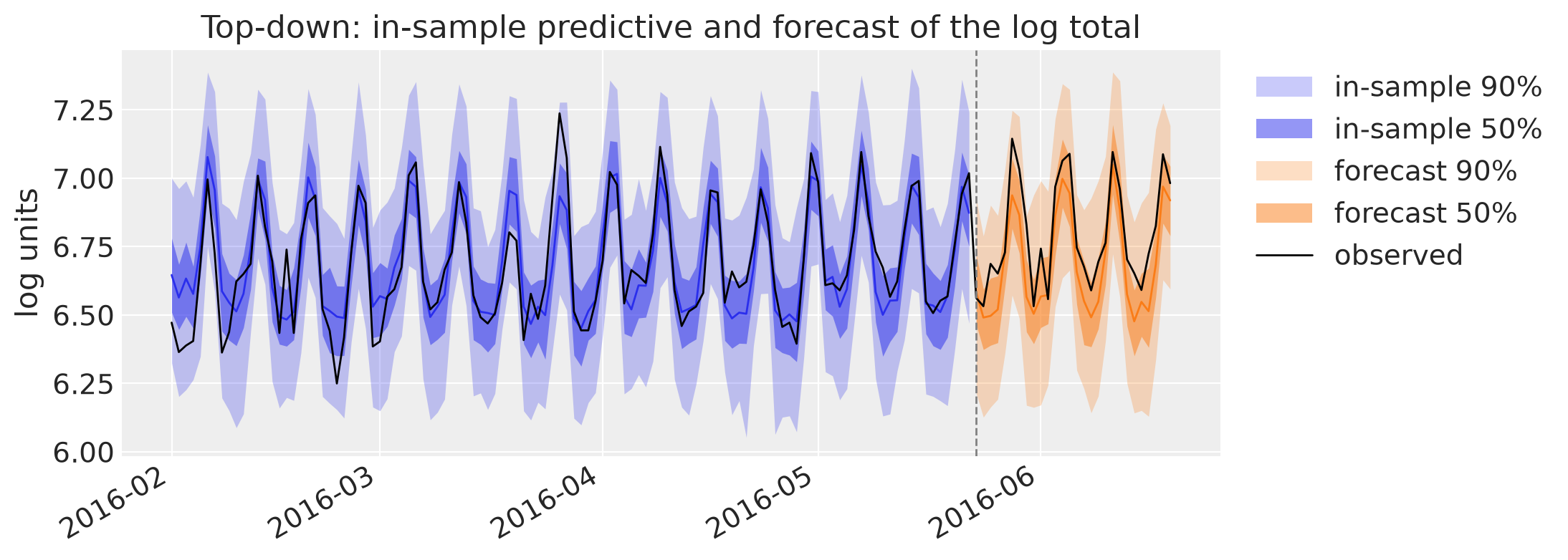
top-down WS-CRPS 0.536, WSPL 0.178
Bottom-up#
Each series borrows its department’s weights inside its store. Two heads, mean and scale, see the same three channels. A bounded exponential keeps an early ADVI step finite,
and a closed day (saled = 0) collapses both heads to the floor \(10^{-3}\):
The observation is \(\mathrm{Gamma}(\alpha = m/\sigma,\ \beta = 1/\sigma)\),
the shape-rate parameterization whose mean is \(m\) and whose variance is
\(m\,\sigma\). Zeros in the data were clamped at \(10^{-3}\) before they entered
y_bottom. predict is given a four-argument factory so the training Gamma
uses the in-sample scale segment and the forecast Gamma uses the future segment.
The latent handed to predict is the mean head; the scale head stays in the
model as the Gamma dispersion. Every weight has the same \(\mathrm{Normal}(0, 1)\)
prior; there are no item-level parameters, so an item is described by its
store-department’s weights and its own moving averages.
def _bounded_exp(x, bound=BEXP_BOUND):
    """Exponential capped at ``bound``. The cap is the ADVI overflow guard."""
    return pt.sigmoid(x - float(np.log(bound))) * bound


class BottomUpModel(ForecastingModel):
    """Department-level mean and scale for every store. Gamma observations."""

    def __init__(self, store_index, dept_index, store_ids, dept_ids):
        self.store_index = np.asarray(store_index, dtype=np.int32)
        self.dept_index = np.asarray(dept_index, dtype=np.int32)
        self.store_ids = tuple(store_ids)
        self.dept_ids = tuple(dept_ids)

    def model(self, covariates, data=None):
        model = pm.modelcontext(None)
        model.add_coord("store", list(self.store_ids))
        model.add_coord("dept", list(self.dept_ids))
        model.add_coord("head", list(HEADS))
        model.add_coord("lag", list(LAGS))
        model.add_coord("day_of_week", list(WEEKDAYS))
        ma_weight = pm.Normal("ma_weight", 0.0, 1.0, dims=("store", "head", "lag", "dept"))
        snap_weight = pm.Normal("snap_weight", 0.0, 1.0, dims=("store", "head", "dept"))
        seasonal = pm.Normal("seasonal", 0.0, 1.0, dims=("store", "day_of_week", "head", "dept"))
        # Weekday is shared, so the first series' channel is the calendar.
        dow = np.asarray(covariates.sel(channel="dow").values)[:, 0].astype(np.int32)
        snap = np.asarray(covariates.sel(channel="snap").values)
        saled = np.asarray(covariates.sel(channel="saled").values)
        log_ma = np.stack(
            [np.asarray(covariates.sel(channel=name).values) for name in LAGS],
            axis=-1,
        )
        store, dept = self.store_index, self.dept_index
        # ma_weight[store, head, lag, dept] -> (series, head, lag), times
        # log_ma (time, series, lag). Sum over the lag axis.
        moving = (ma_weight[store, :, :, dept][None] * log_ma[:, :, None, :]).sum(-1)
        snap_effect = snap_weight[store, :, dept][None] * snap[:, :, None]
        # (series, weekday, head) indexed by this day's weekday is
        # (series, time, head). Time has to lead.
        seasonal_effect = seasonal[store, :, :, dept][:, dow, :].transpose(1, 0, 2)
        combined = moving + snap_effect + seasonal_effect
        mean = _bounded_exp(combined[..., 0]) * saled + GAMMA_FLOOR
        scale = _bounded_exp(combined[..., 1]) * saled + GAMMA_FLOOR
        t_obs = self.horizon.t_obs

        def gamma(name, latent, dims, observed):
            scale_seg = scale[t_obs:] if name == FORECAST_VAR else scale[:t_obs]
            return pm.Gamma(
                name,
                alpha=latent / scale_seg,
                beta=1.0 / scale_seg,
                dims=dims,
                observed=observed,
            )

        self.predict(gamma, mean)
bottom_model = BottomUpModel(store_index, dept_index, store_ids, dept_ids)
cov_bottom_fit = cov_bottom.isel({TIME_DIM: slice(T0, None)})
bottom, bottom_posterior, bottom_forecast, bottom_seconds = fit_and_forecast(
    bottom_model, y_bottom, cov_bottom_fit, STEPS["bottom-up"]
)
plot_loss(bottom.losses, f"Bottom-up ELBO ({STEPS['bottom-up']} steps, {bottom_seconds:.1f} s)")
bottom_draws = reconcile_bottom_up(bottom_forecast, ORIGIN)
bottom_scores, bottom_wspl = score_holdout(bottom_draws)
results["bottom-up"] = {
    "scores": bottom_scores,
    "wspl": bottom_wspl,
    "seconds": bottom_seconds,
    "draws": bottom_draws,
}
print(f"bottom-up WS-CRPS {mean_level_score(bottom_scores):.3f}, WSPL {bottom_wspl:.3f}")
/var/folders/cm/3dzy9rdd5s3672z0s1brjkvh0000gn/T/ipykernel_69810/3881171391.py:27: UserWarning: The figure layout has changed to tight
  fig.tight_layout()
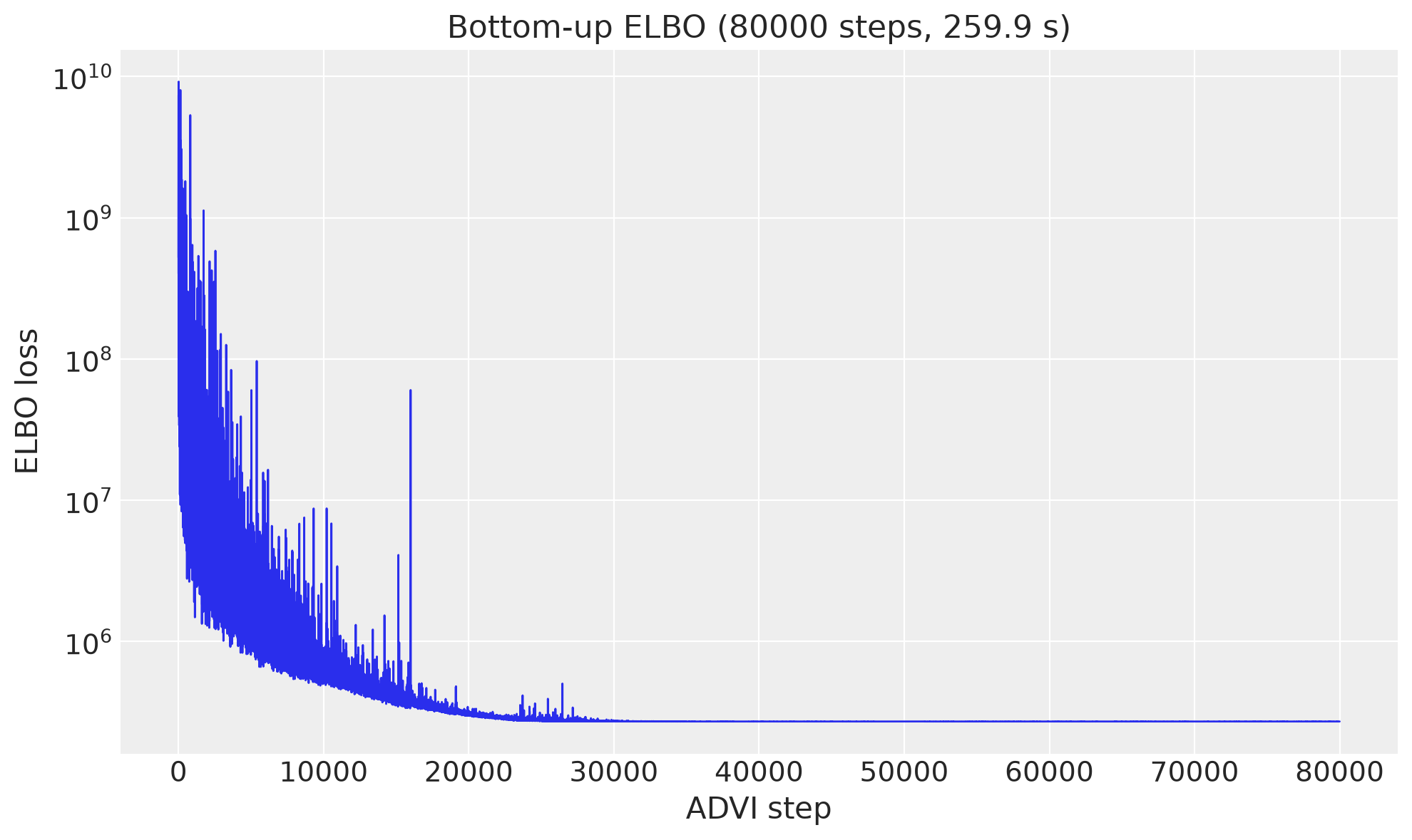
bottom-up WS-CRPS 0.722, WSPL 0.241
pc = az.plot_forest(
    bottom_posterior.sel(head="mean"),
    var_names=["snap_weight"],
    combined=True,
    figure_kwargs={"figsize": (8, 7)},
)
pc.viz["figure"].item().suptitle(
    "Bottom-up: SNAP effect on the log mean, by store and department", fontsize=13
)
ma_sum = bottom_posterior["ma_weight"].sel(head="mean").sum("lag")
display(
    ma_sum.mean(("chain", "draw"))
    .to_pandas()
    .round(2)
    .rename_axis(index="store", columns="sum of MA weights (mean head)")
)
| sum of MA weights (mean head) | FOODS_1 | FOODS_2 | FOODS_3 | HOBBIES_1 | HOBBIES_2 | HOUSEHOLD_1 | HOUSEHOLD_2 |
|---|---|---|---|---|---|---|---|
| store | |||||||
| CA_1 | 0.39 | 0.22 | 0.19 | 0.20 | 0.09 | 0.40 | 0.41 |
| CA_2 | 0.61 | 0.18 | 0.19 | 0.23 | 0.06 | 0.15 | 0.38 |
| TX_1 | 0.76 | 0.21 | 0.22 | 0.20 | 0.19 | 0.03 | 0.36 |
| WI_1 | 0.62 | 0.13 | 0.20 | 0.27 | 0.10 | -0.01 | 0.21 |
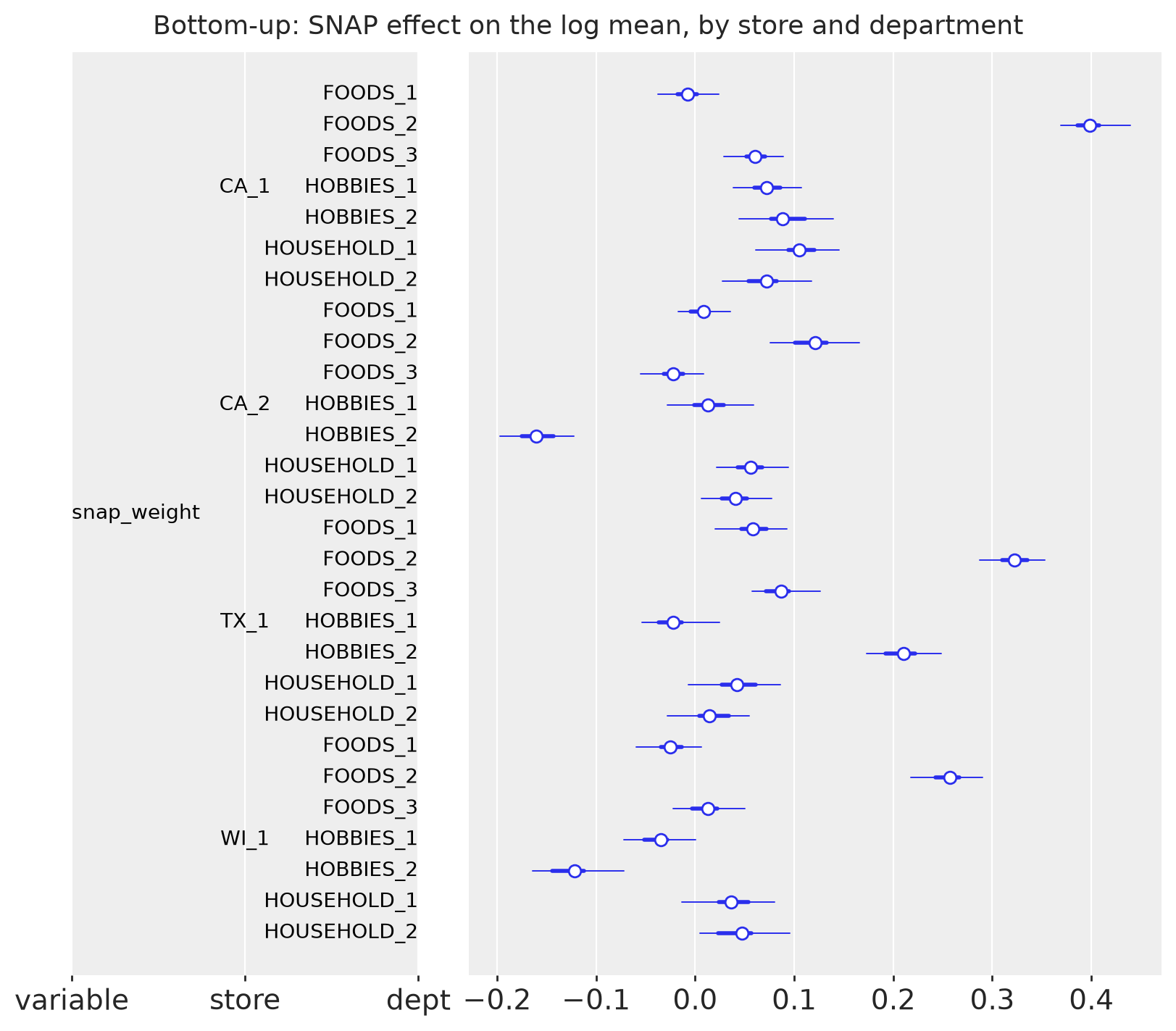
The SNAP effect on the log mean is a food effect, as numpyro_forecast finds on
the full panel: FOODS_2 has the largest coefficient in every store (0.12 in
CA_2 to 0.40 in CA_1, a 13% to 50% lift on a SNAP day), the other food
departments stay below 0.1, and the hobbies and household departments scatter
around zero with the widest intervals on HOBBIES_2, the department with the
fewest units. The table is the sum of the three moving-average weights of the
mean head, the exponent the model applies to an item’s recent level: between
0.4 and 0.8 for FOODS_1, 0.1 to 0.4 for most other departments, and about zero
for HOUSEHOLD_1 in TX_1 and WI_1, where the weekday and SNAP effects carry
the whole regression. Every exponent is well below one, so the model shrinks a
best seller toward its store-department and lifts a slow one, which is the
reason for its item-level scores below.
Middle-out#
Level 9 is store by department. Each of those series was divided by its own
training-window scale before it became y_mid. Each series then has its own
regression and its own noise scale. The degrees of freedom are shared:
with \(f_{t,1..104}\) the sine and cosine of the 52 yearly harmonics. \(b_g \sim \mathrm{Normal}(0, 10)\), \(\tau_g \sim \mathrm{LogNormal}(-1, 1)\), the Fourier weights are \(\mathrm{Normal}(0, 1)\), the weekday effect is \(\mathrm{Normal}(0, 1)\), the noise scale is \(\mathrm{LogNormal}(-1, 1)\), and \(\nu \sim \mathrm{Uniform}(1, 10)\). The forecast is clipped at zero, multiplied back by the training scale, and split to the items of the group.
class MiddleOutModel(ForecastingModel):
    """One scaled regression per series. Shared Student-T degrees of freedom."""

    def model(self, covariates, data=None):
        years = np.asarray(covariates.sel(feature="years").values)[:, None]
        dow = np.asarray(covariates.sel(feature="dow").values).astype(np.int32)
        fourier_names = [
            str(name)
            for name in covariates.coords["feature"].values
            if str(name).startswith(("sin_", "cos_"))
        ]
        feature = np.asarray(covariates.sel(feature=fourier_names).values, dtype=np.float64)
        model = pm.modelcontext(None)
        model.add_coord("day_of_week", list(WEEKDAYS))
        model.add_coord("fourier", fourier_names)
        bias = pm.Normal("bias", 0.0, 10.0, dims="series")
        trend = pm.LogNormal("trend", -1.0, 1.0, dims="series")
        weight = pm.Normal("weight", 0.0, 1.0, dims=("series", "fourier"))
        seasonal = pm.Normal("seasonal", 0.0, 1.0, dims=("day_of_week", "series"))
        noise_scale = pm.LogNormal("noise_scale", -1.0, 1.0, dims="series")
        dof = pm.Uniform("dof", 1.0, 10.0)
        prediction = bias + trend * years + seasonal[dow] + pt.dot(feature, weight.T)
        self.predict(pm.StudentT.dist(nu=dof, mu=0.0, sigma=noise_scale), prediction)
middle, middle_posterior, middle_forecast, middle_seconds = fit_and_forecast(
    MiddleOutModel(), y_mid, cov_mid, STEPS["middle-out"]
)
plot_loss(
    middle.losses,
    f"Middle-out ELBO ({STEPS['middle-out']} steps, {middle_seconds:.1f} s)",
)
display(az.summary(middle_posterior, var_names=["dof"]))
first_store = [label for label in level9_labels if label.startswith(f"{store_ids[0]}/")]
pc = az.plot_forest(
    middle_posterior.sel(series=first_store),
    var_names=["trend", "noise_scale"],
    combined=True,
    figure_kwargs={"figsize": (8, 5)},
)
pc.viz["figure"].item().suptitle(
    f"Middle-out: trend and noise scale by department, store {store_ids[0]} "
    "(in typical daily changes)",
    fontsize=13,
);
/var/folders/cm/3dzy9rdd5s3672z0s1brjkvh0000gn/T/ipykernel_69810/3881171391.py:27: UserWarning: The figure layout has changed to tight
  fig.tight_layout()
| mean | sd | hdi94_lb | hdi94_ub | ess_bulk | ess_tail | r_hat | mcse_mean | mcse_sd | |
|---|---|---|---|---|---|---|---|---|---|
| dof | 3.473 | 0.039 | 3.4 | 3.5 | 142 | 183 | nan | 0.0032 | 0.0022 |
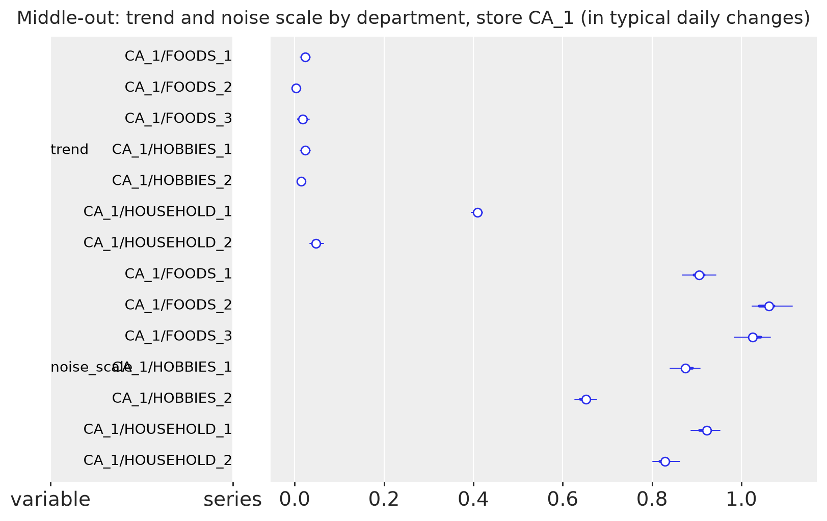
The degrees of freedom shared by the 28 series come out at about 3.5 with a tight
interval: heavier tails than numpyro_forecast’s 6.5 on the 70 full
store-departments, because three items per store-department leave more spikes
and zeros than 435 do. The trends are near zero (the series are flat), except
HOUSEHOLD_1, which grows by 0.4 typical daily changes a year in CA_1. The
noise scales sit between 0.65 and 1.05 typical daily changes, so the calendar
explains part of the day-to-day movement for every department and most of it
for none; HOBBIES_2, the smallest department, is the most predictable in these
units because its scale is the smallest.
middle_in_sample = forecast_draws(
    middle.predict_in_sample(posterior=middle_posterior, random_seed=SEED)["posterior_predictive"][
        "obs"
    ]
)
middle_future = forecast_draws(middle_forecast)
columns = [level9_labels.index(label) for label in first_store]
fig, axes = plt.subplots(
    len(columns), 1, figsize=(11, 2.2 * len(columns)), sharex=True, layout="constrained"
)
for ax, k in zip(axes, columns, strict=True):
    plot_window(
        ax,
        middle_in_sample[..., k] * scale_mid[k],
        np.clip(middle_future[..., k], 0.0, None) * scale_mid[k],
        level9[:, k],
        title=level9_labels[k],
        ylabel="units",
    )
handles, labels = axes[0].get_legend_handles_labels()
fig.legend(handles, labels, loc="outside lower center", ncols=5)
fig.suptitle(f"Middle-out: in-sample predictive and forecast, store {store_ids[0]}", fontsize=14)
plt.show()

middle_draws = reconcile_middle_out(middle_forecast, ORIGIN)
middle_scores, middle_wspl = score_holdout(middle_draws)
results["middle-out"] = {
    "scores": middle_scores,
    "wspl": middle_wspl,
    "seconds": middle_seconds,
    "draws": middle_draws,
}
print(f"middle-out WS-CRPS {mean_level_score(middle_scores):.3f}, WSPL {middle_wspl:.3f}")
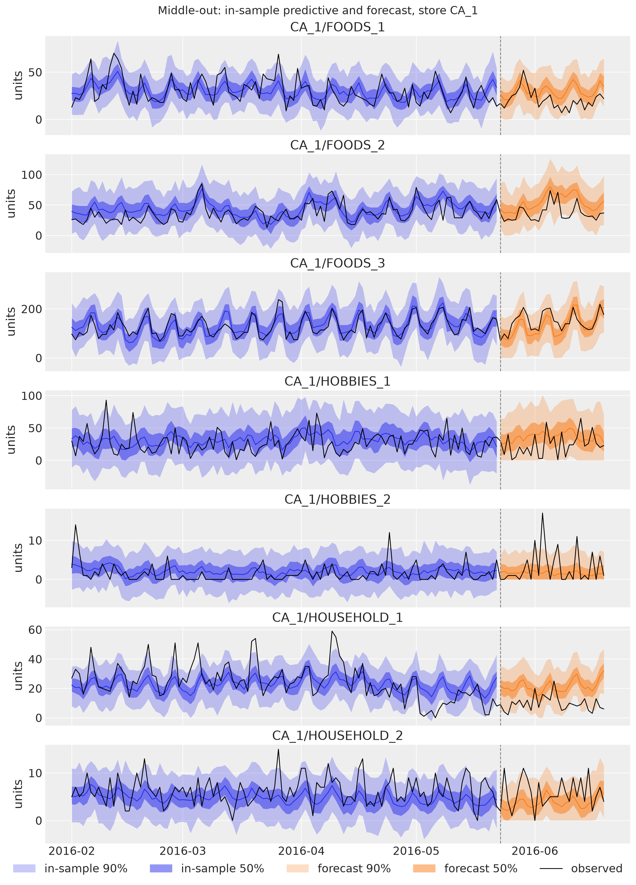
middle-out WS-CRPS 0.732, WSPL 0.248
The fit follows the weekly pattern of the food departments and the forecast
continues it; the bands have a constant width per series (the noise scale times
the series scale), because the model has no latent state. HOUSEHOLD_1 shows the
weakness of a positive-trend regression: its sales drop in the last training
month and the forecast stays at the level of the trend, above the observations
for the whole holdout.
Backtest#
The kit backtests on three 28-day windows inside the training period, 35 days
apart (origins at days 1,843, 1,878 and 1,913), refitting on all the data before
each origin. backtest does the same with min_train_window, test_window and
stride, fitting a fresh Forecaster per window with its own seed. Each model
is handed the series it trains on (the log total, the scaled level-9 sums, or the
clamped counts from day 121); the transform hook reconciles the window’s
forecast to the 84 items with the shares of that window’s last 28 training days
and sums draws and truth to the 12 levels, and per_window_metrics builds the
twelve weighted scaled CRPS metrics with the weights and scales of that origin.
The bottom-up series starts at day 121, so its window positions are offset by
T0 when the weights and scales are built.
def run_backtest(name, model, data, covariates, reconcile, *, offset=0):
    """Three expanding-window backtests of one model, scored on the 12 levels."""
    duration = data.sizes[TIME_DIM]

    def transform(pred, truth):
        origin = int(np.flatnonzero(time == truth[FUTURE_DIM].values[0])[0])
        bottom = reconcile(pred, origin)
        truth_levels = aggregate(panel_sales[origin : origin + HORIZON], panel.matrix)
        return aggregate(bottom, panel.matrix), truth_levels

    started = perf_counter()
    windows = backtest(
        data,
        covariates.sel({TIME_DIM: data[TIME_DIM].values}),
        model,
        metrics={},
        per_window_metrics=partial(m5_window_metrics, offset=offset),
        transform=transform,
        min_train_window=duration - HORIZON - (N_BACKTEST - 1) * STRIDE,
        test_window=HORIZON,
        stride=STRIDE,
        num_samples=SAMPLES,
        forecaster_options={"num_steps": STEPS[name], "backend": BACKEND, "progressbar": False},
        random_seed=SEED,
    )
    print(f"{name}: {len(windows)} windows in {perf_counter() - started:.0f} s")
    frame = results_to_dataframe(windows)
    level_columns = [f"ws_crps_{level}" for level in LEVELS]
    return frame.assign(
        model=name,
        origin=frame["t1"] + offset,
        ws_crps=frame[level_columns].mean(axis=1),
    )


backtest_df = pd.concat(
    [
        run_backtest("top-down", TopDownModel(), y_top, cov_top, reconcile_top_down),
        run_backtest(
            "bottom-up", bottom_model, y_bottom, cov_bottom_fit, reconcile_bottom_up, offset=T0
        ),
        run_backtest("middle-out", MiddleOutModel(), y_mid, cov_mid, reconcile_middle_out),
    ],
    ignore_index=True,
)
assert sorted(backtest_df["origin"].unique()) == sorted(
    ORIGIN - HORIZON - k * STRIDE for k in range(N_BACKTEST)
)
display(
    backtest_df[["model", "origin", "train_walltime", "ws_crps"]].round(
        {"train_walltime": 1, "ws_crps": 3}
    )
)
top-down: 3 windows in 8 s
bottom-up: 3 windows in 651 s
middle-out: 3 windows in 92 s
| model | origin | train_walltime | ws_crps | |
|---|---|---|---|---|
| 0 | top-down | 1843 | 2.2 | 0.460 |
| 1 | top-down | 1878 | 2.4 | 0.494 |
| 2 | top-down | 1913 | 2.4 | 0.447 |
| 3 | bottom-up | 1843 | 236.5 | 0.615 |
| 4 | bottom-up | 1878 | 207.3 | 0.652 |
| 5 | bottom-up | 1913 | 201.3 | 0.607 |
| 6 | middle-out | 1843 | 29.9 | 0.653 |
| 7 | middle-out | 1878 | 30.1 | 0.591 |
| 8 | middle-out | 1913 | 31.0 | 0.567 |
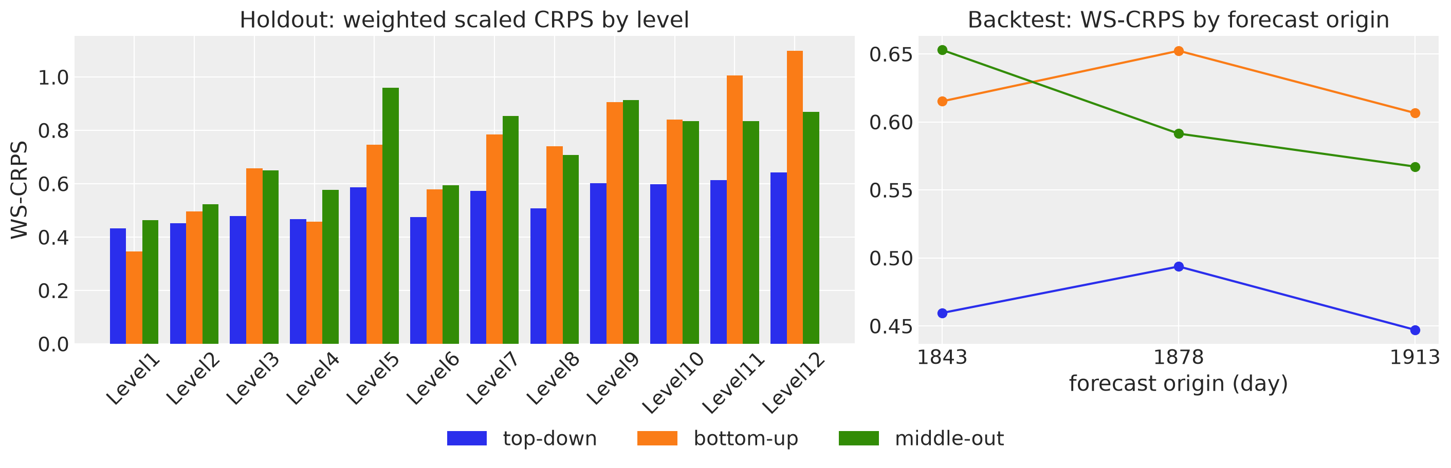
The top-down model scores best in every window, by a wide margin (0.45 to 0.49 against 0.57 to 0.65). The other two swap places: bottom-up is ahead at the first origin, middle-out at the later two, and middle-out improves from window to window while bottom-up does not. That is the ranking numpyro_forecast reports on the full panel (top-down, then middle-out, then bottom-up in every window), with the two split models closer together here.
What the three forecasts say about this panel#
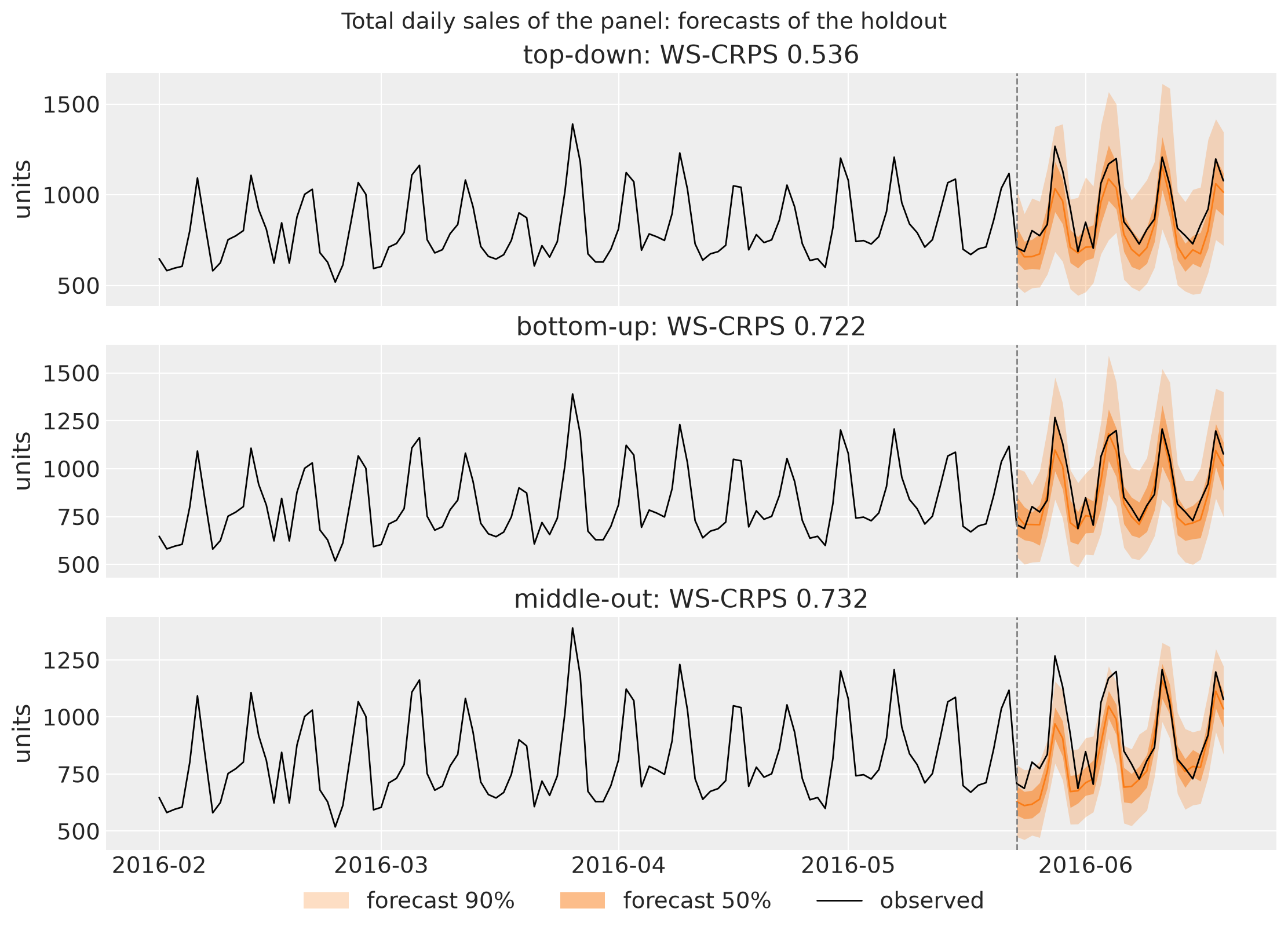
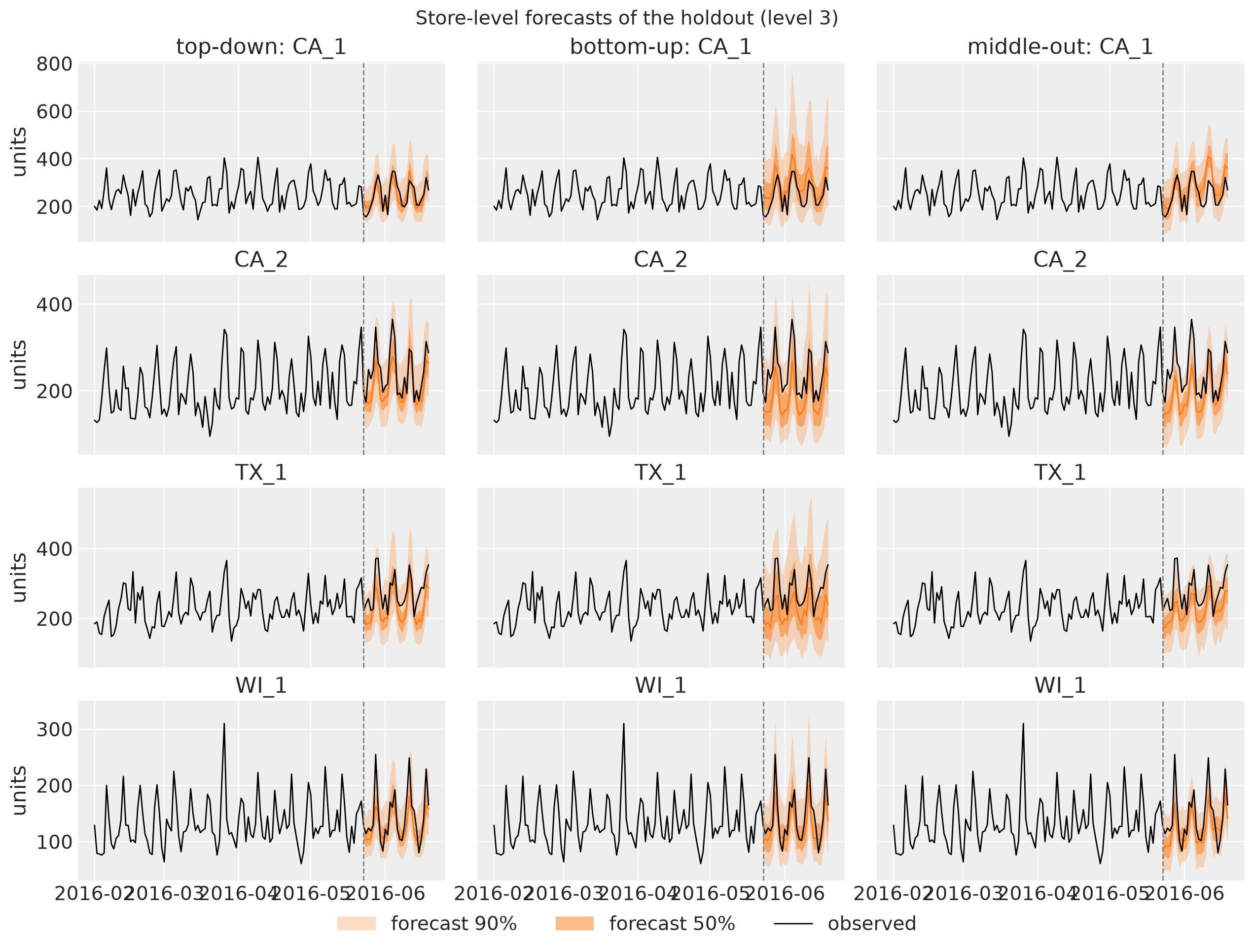
The table lists the holdout scores of the three final fits, the mean of their three backtest scores, and two calibration numbers at the total level: the ratio of the median forecast to the observed holdout mean (1 is unbiased) and the share of holdout days inside the 90% band (0.9 is calibrated). The bands below are the total of the reconciled bottom draws over the holdout, then the same forecasts at the four stores, the per-level scores of the holdout, and the backtest scores by origin. None of these numbers are competition scores: the panel is 84 series, and mean-field ADVI is not the kit’s optimizer.
holdout_total = panel_sales[ORIGIN:end].sum(-1)


def total_calibration(draws):
    """Median-to-truth ratio and 90% coverage of the total-level forecast."""
    total = np.asarray(draws).sum(-1)
    low, high = np.quantile(total, [0.05, 0.95], axis=0)
    return {
        "total median / truth": float(np.median(total, axis=0).mean() / holdout_total.mean()),
        "total 90% coverage": float(((holdout_total >= low) & (holdout_total <= high)).mean()),
    }


summary = pd.DataFrame(
    [
        {
            "model": name,
            "ws_crps": mean_level_score(payload["scores"]),
            "wspl": payload["wspl"],
            "backtest ws_crps": backtest_df.loc[backtest_df["model"] == name, "ws_crps"].mean(),
            **total_calibration(payload["draws"]),
            "fit_seconds": payload["seconds"],
        }
        for name, payload in results.items()
    ]
)
display(summary.round(3))

fig, axes = plt.subplots(3, 1, figsize=(11, 8), sharex=True, layout="constrained")
for ax, (name, payload) in zip(axes, results.items(), strict=True):
    plot_window(
        ax,
        None,
        np.asarray(payload["draws"]).sum(-1),
        panel_sales.sum(-1),
        title=f"{name}: WS-CRPS {mean_level_score(payload['scores']):.3f}",
        ylabel="units",
    )
handles, labels = axes[0].get_legend_handles_labels()
fig.legend(handles, labels, loc="outside lower center", ncols=3)
fig.suptitle("Total daily sales of the panel: forecasts of the holdout", fontsize=14)
plt.show()
| model | ws_crps | wspl | backtest ws_crps | total median / truth | total 90% coverage | fit_seconds | |
|---|---|---|---|---|---|---|---|
| 0 | top-down | 0.536 | 0.178 | 0.467 | 0.900 | 1.000 | 5.277 |
| 1 | bottom-up | 0.722 | 0.241 | 0.625 | 0.944 | 1.000 | 259.877 |
| 2 | middle-out | 0.732 | 0.248 | 0.604 | 0.906 | 0.786 | 36.897 |
store_slice = panel.slices["Level3"]
store_truth = aggregate(panel_sales, panel.matrix)[:, store_slice]
fig, axes = plt.subplots(
    len(store_ids),
    len(results),
    figsize=(4.2 * len(results), 2.4 * len(store_ids)),
    sharex=True,
    sharey="row",
    layout="constrained",
)
for column, (name, payload) in enumerate(results.items()):
    store_draws = aggregate(payload["draws"], panel.matrix)[..., store_slice]
    for row, store in enumerate(store_ids):
        plot_window(
            axes[row, column],
            None,
            store_draws[..., row],
            store_truth[:, row],
            title=f"{name}: {store}" if row == 0 else store,
            ylabel="units" if column == 0 else "",
        )
handles, labels = axes[0, 0].get_legend_handles_labels()
fig.legend(handles, labels, loc="outside lower center", ncols=3)
fig.suptitle("Store-level forecasts of the holdout (level 3)", fontsize=14)
plt.show()
level_scores = pd.DataFrame({name: payload["scores"] for name, payload in results.items()}).T
display(level_scores.round(3))

level_columns = [f"ws_crps_{level}" for level in LEVELS]
fig, axes = plt.subplots(1, 2, figsize=(14, 4.5), width_ratios=[3, 2], layout="constrained")
x = np.arange(len(LEVELS))
width = 0.27
for k, (name, payload) in enumerate(results.items()):
    axes[0].bar(
        x + (k - 1) * width, [payload["scores"][level] for level in LEVELS], width, label=name
    )
axes[0].set_xticks(x, list(LEVELS), rotation=45)
axes[0].set(title="Holdout: weighted scaled CRPS by level", ylabel="WS-CRPS")
for name in results:
    rows = backtest_df[backtest_df["model"] == name].sort_values("origin")
    axes[1].plot(rows["origin"], rows["ws_crps"], marker="o", label=name)
axes[1].set(title="Backtest: WS-CRPS by forecast origin", xlabel="forecast origin (day)")
axes[1].set_xticks(sorted(backtest_df["origin"].unique()))
handles, labels = axes[0].get_legend_handles_labels()
fig.legend(handles, labels, loc="outside lower center", ncols=3)
plt.show()
| Level1 | Level2 | Level3 | Level4 | Level5 | Level6 | Level7 | Level8 | Level9 | Level10 | Level11 | Level12 | |
|---|---|---|---|---|---|---|---|---|---|---|---|---|
| top-down | 0.433 | 0.452 | 0.480 | 0.467 | 0.587 | 0.474 | 0.572 | 0.508 | 0.601 | 0.597 | 0.613 | 0.643 |
| bottom-up | 0.347 | 0.496 | 0.657 | 0.459 | 0.747 | 0.579 | 0.785 | 0.740 | 0.905 | 0.841 | 1.005 | 1.098 |
| middle-out | 0.463 | 0.524 | 0.650 | 0.577 | 0.959 | 0.595 | 0.854 | 0.708 | 0.914 | 0.835 | 0.834 | 0.868 |
Discussion#
Top-down scores best, on the holdout (WS-CRPS 0.54 against 0.72 and 0.73) and in every backtest window, as it does for numpyro_forecast on the full panel. One Student-T regression on the total has the fewest parameters and the most data per parameter, and the share split carries that forecast down the hierarchy as long as the item shares are stable over four weeks. It leads at every level except the total and the categories, where bottom-up is a little ahead on this holdout.
Bottom-up and middle-out are close behind each other and far behind top-down. Bottom-up loses at the item levels (10 to 12), where every intermittent series has to be right on its own and the department-level exponent of 0.1 to 0.8 shrinks the best sellers, which carry the dollar weights. Middle-out loses most at the category and department levels (4 to 7), the sums of its 28 independent regressions: no information is shared across stores, and the 104 Fourier weights per series with unit priors fit five Junes better than the next one. Averaged over the backtest windows middle-out is ahead (0.60 against 0.63); on the holdout the two are tied.
All three forecast the total a little low (median 0.90 to 0.94 of the observed mean): the holdout is the four weeks before Memorial Day, when the observed total runs above the training level. Top-down and bottom-up cover the holdout with their 90% bands on every day; the middle-out bands, the sum of 28 clipped Student-T noises, miss on a fifth of the days. The bottom-up bands at the total are not too narrow here, unlike numpyro_forecast’s 30,490-series sum: with 84 Gamma draws per day the independent noise does not average out.
Item levels 10 to 12 of top-down and middle-out are not model forecasts: they are the share heuristic with Poisson noise, which is what the kit submits. That the heuristic beats the bottom-up model there says more about the bottom-up model than about the split.
What is not comparable to numpyro_forecast: the scores (84 series against 30,490, different weights and scales), the posterior draws (mean-field ADVI at a fixed learning rate against clipped SVI with a decaying one), and the middle-out scale (one scale per series for the whole notebook against one per backtest window). The data pipeline is: the official weights match on all 42,840 aggregates, and the hierarchy, scales, shares and Poisson split reproduce the upstream functions to floating-point precision.
Next steps#
Give the bottom-up model a count likelihood (
pm.NegativeBinomial) and an item-level intercept, and compare the item-level scores again.Add a random-walk level to the top-down and middle-out regressions with
innovations, as the kit’s forecasting tutorials do for the same data.Reconcile the three forecasts with MinT-style weights instead of picking one strategy.
References#
Pyro team, Pyro M5 starter kit (
model1.py,model2.py,model3.py,evaluate.py).Upstream notebook: https://juanitorduz.github.io/numpyro_forecast/docs/examples/m5_forecasting.html.
Makridakis, S., Spiliotis, E., Assimakopoulos, V., Chen, Z., Gaba, A., Tsetlin, I., Winkler, R. L. (2022). The M5 uncertainty competition: Results, findings and conclusions. International Journal of Forecasting, 38(4).
Hyndman & Athanasopoulos, Forecasting: Principles and Practice, hierarchical forecasting.
M5 competition: https://www.kaggle.com/c/m5-forecasting-uncertainty/overview.
Nixtla, m5-forecasts (the data mirror).