Intermittent demand: genuine zeros, stockouts and availability scenarios

A zero can mean that nobody wanted a product or that it was unavailable. We model these mechanisms explicitly with a Bernoulli occurrence process and a Gamma positive quantity. This is a hurdle model for continuous quantities such as kg; for integer unit sales use an appropriate positive count distribution instead.

This is a generative alternative inspired by Juan Orduz’s TSB and availability TSB examples. It is not a literal TSB implementation: time-varying occurrence probabilities are regression parameters, and each forecast samples an actual occurrence and quantity. The additive-error ssoe helper in the ARMA example serves a different model family.

Prepare notebook

import os

import arviz as az
import matplotlib.pyplot as plt
import numpy as np
import pandas as pd
import pymc as pm
import pytensor.tensor as pt
import xarray as xr

from pymc_forecast import (
    HMCForecaster,
    Horizon,
    evaluate_forecast,
    predict,
)

SMOKE = os.getenv("PYMC_FORECAST_SMOKE_TEST") == "1"
SEED = 2026
rng = np.random.default_rng(SEED)
DRAWS, TUNE, CHAINS = (25, 25, 1) if SMOKE else (600, 800, 2)
N_PRED = 50 if SMOKE else 800
HDI_PROB = 0.94

az.style.use("arviz-darkgrid")
if "stats.ci_kind" in az.rcParams:  # ArviZ 1.x; ArviZ 0.x intervals are always HDI
    az.rcParams["stats.ci_kind"] = "hdi"
az.rcParams["stats.ci_prob"] = HDI_PROB
plt.rcParams["figure.figsize"] = [10, 6]
plt.rcParams["figure.dpi"] = 100
plt.rcParams["figure.facecolor"] = "white"

%config InlineBackend.figure_format = "retina"
print(
    "Execution mode:", "CI smoke check; do not interpret fit quality" if SMOKE else "full example"
)

Execution mode: full example

Simulate demand before observing sales

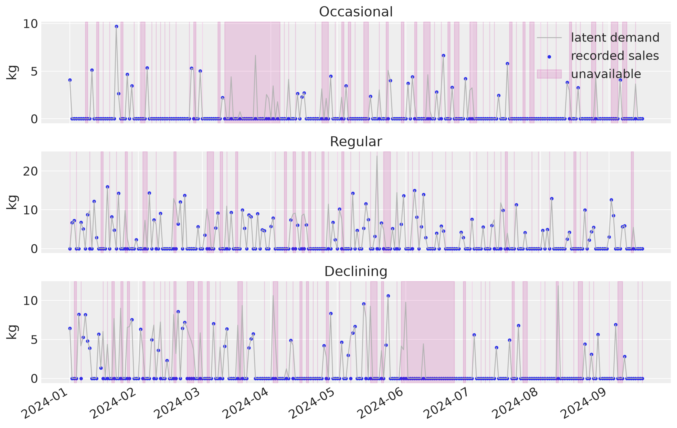
Three products have different demand frequencies. The third gradually loses demand. Availability is simulated independently of latent demand here, so stockout periods provide no evidence about the occurrence probability. Real stockouts caused by high demand require an inventory/censoring model; this example assumes a known external availability mask and no partial-day capacity cap.

n_train, horizon = 220, 40
n = n_train + horizon
products = ["Occasional", "Regular", "Declining"]
time = pd.date_range("2024-01-01", periods=n, freq="D")
t_scaled = np.arange(n) / n_train
intercept = np.array([-1.3, -0.2, 0.3])
slope = np.array([0.0, 0.0, -2.2])
probability = 1 / (1 + np.exp(-(intercept + t_scaled[:, None] * slope)))
size_mean = np.array([4.0, 8.0, 6.0])
shape = 5.0
latent_demand = (rng.random((n, 3)) < probability) * rng.gamma(shape, size_mean / shape, (n, 3))
availability = (rng.random((n, 3)) > np.array([0.4, 0.3, 0.35])).astype(float)
availability[70:95, 0] = 0
availability[150:175, 2] = 0
sales = xr.DataArray(
    availability * latent_demand,
    dims=("time", "product"),
    coords={"time": time, "product": products},
)
inputs = xr.DataArray(
    np.stack([np.broadcast_to(t_scaled[:, None], (n, 3)), availability], axis=1),
    dims=("time", "input", "product"),
    coords={"time": time, "input": ["elapsed", "available"], "product": products},
)
train = sales.isel(time=slice(n_train))
train_inputs = inputs.isel(time=slice(n_train))
truth_sales = sales.isel(time=slice(n_train, None)).rename(time="time_future")
truth_demand = xr.DataArray(
    latent_demand[n_train:],
    dims=("time_future", "product"),
    coords={"time_future": time[n_train:], "product": products},
)
fig, axes = plt.subplots(3, 1, figsize=(11, 7), sharex=True)
for j, ax in enumerate(axes):
    ax.plot(time, latent_demand[:, j], color="0.7", lw=1, label="latent demand")
    ax.scatter(time, sales[:, j], s=9, label="recorded sales")
    ax.fill_between(
        time,
        0,
        1,
        where=availability[:, j] == 0,
        transform=ax.get_xaxis_transform(),
        color="C3",
        alpha=0.15,
        label="unavailable",
    )
    ax.set(ylabel="kg", title=products[j])
axes[0].legend(loc="upper right")
fig.autofmt_xdate()
fig.tight_layout()
plt.show()

/var/folders/cm/3dzy9rdd5s3672z0s1brjkvh0000gn/T/ipykernel_69767/107458588.py:50: UserWarning: The figure layout has changed to tight
  fig.tight_layout()

Model occurrence and positive quantity separately

For product \(s\), \(p_{t,s}=\operatorname{sigmoid}(a_s+b_s t)\) and \(Y_{t,s}\sim\operatorname{HurdleGamma}(\psi=A_{t,s}p_{t,s},m_s,k_s)\). Thus \(E[Y_{t,s}]=A_{t,s}p_{t,s}m_s\). At zero availability the observation is certainly zero and contributes no information about demand. At full availability, zeros are genuine non-occurrence events. The probability always lies in \([0,1]\), and positive quantities are never negative.

The model receives named inputs; the only future values it reads are elapsed time and the availability scenario. predict receives the expected sales on the outcome scale, which makes its mu_future output directly interpretable in kg.

def demand_model(covariates, data=None):
    h = Horizon.from_data(covariates, data)
    elapsed = pt.as_tensor_variable(covariates.sel(input="elapsed").values)
    available = pt.as_tensor_variable(covariates.sel(input="available").values)
    intercept = pm.Normal("occurrence_intercept", 0, 1.5, dims="product")
    slope = pm.Normal("occurrence_slope", 0, 1.5, dims="product")
    size_mean = pm.LogNormal("positive_mean", np.log(5), 0.8, dims="product")
    shape = pm.LogNormal("positive_shape", np.log(4), 0.6, dims="product")
    psi = available * pm.math.sigmoid(intercept + elapsed * slope)
    expectation = psi * size_mean

    def likelihood(name, expected, dims, observed):
        segment = slice(0, h.t_obs) if dims[0] == "time" else slice(h.t_obs, None)
        return pm.HurdleGamma(
            name,
            psi=psi[segment],
            alpha=shape,
            beta=shape / size_mean,
            dims=dims,
            observed=observed,
        )

    predict(h, likelihood, expectation)


fc = HMCForecaster(
    demand_model,
    train,
    train_inputs,
    draws=DRAWS,
    tune=TUNE,
    chains=CHAINS,
    random_seed=SEED,
    progressbar=False,
    sample_kwargs={"target_accept": 0.9},
)
az.summary(fc.idata, var_names=["occurrence_intercept", "occurrence_slope", "positive_mean"])

Initializing NUTS using jitter+adapt_diag...

Multiprocess sampling (2 chains in 2 jobs)

NUTS: [occurrence_intercept, occurrence_slope, positive_mean, positive_shape]

Sampling 2 chains for 800 tune and 600 draw iterations (1_600 + 1_200 draws total) took 2 seconds.

We recommend running at least 4 chains for robust computation of convergence diagnostics

	mean	sd	hdi94_lb	hdi94_ub	ess_bulk	ess_tail	r_hat	mcse_mean	mcse_sd
occurrence_intercept[Occasional]	-1.11	0.37	-1.9	-0.5	1157	1005	1.00	0.011	0.01
occurrence_intercept[Regular]	-0.01	0.3	-0.58	0.54	1178	761	1.00	0.0088	0.0088
occurrence_intercept[Declining]	-0.15	0.34	-0.74	0.51	1431	944	1.00	0.0091	0.0098
occurrence_slope[Occasional]	-0.44	0.66	-1.6	0.82	1221	953	1.00	0.019	0.017
occurrence_slope[Regular]	-0.48	0.52	-1.4	0.54	1374	1005	1.00	0.014	0.014
occurrence_slope[Declining]	-1.66	0.65	-2.9	-0.48	1535	915	1.00	0.017	0.021
positive_mean[Occasional]	4.15	0.35	3.5	4.8	1606	755	1.00	0.0088	0.011
positive_mean[Regular]	7.56	0.44	6.8	8.4	1490	779	1.00	0.012	0.015
positive_mean[Declining]	5.73	0.39	5	6.5	1520	731	1.00	0.01	0.013

Two scenarios from the same posterior

We use the simulated future availability as a specified scenario, not as information that would ordinarily be known at ordering time. Full availability describes latent unconstrained demand under this model. Both calls use identical parameter draws; we compare conditional means to avoid adding Monte Carlo observation noise to the scenario difference.

posterior = fc.draw_posterior(N_PRED, random_seed=SEED + 1)
future_inputs = inputs.isel(time=slice(n_train, None))
full_inputs = future_inputs.copy(deep=True)
full_inputs.loc[{"input": "available"}] = 1.0
planned = fc.forecast(
    future_covariates=future_inputs, posterior=posterior, random_seed=SEED + 2
).predictions
full = fc.forecast(
    future_covariates=full_inputs, posterior=posterior, random_seed=SEED + 3
).predictions
assert full.forecast.dims == ("chain", "draw", "time_future", "product")
assert bool((full.forecast >= 0).all())
assert bool((full.forecast == 0).any())
assert bool((full.forecast > 0).any())
mask = future_inputs.sel(input="available").rename(time="time_future")
np.testing.assert_allclose(planned.mu_future, full.mu_future * mask)
assert bool((planned.forecast.where(mask == 0, 0) == 0).all())

expected_lost = (full.mu_future - planned.mu_future).sum("time_future")
expected_lost.quantile([0.05, 0.5, 0.95], dim=("chain", "draw")).to_pandas()

/Users/juanitorduz/.paseo/worktrees/1dtaxlkh/docs-example-notebook-visual-style/.venv/lib/python3.14/site-packages/pymc/distributions/mixture.py:311: MixtureTransformWarning: No safe default transform found for Mixture distribution forecast. This can happen when components have different supports or default transforms.
If appropriate, you can specify a custom transform for more efficient sampling.
  transform_warning()

Sampling: [forecast]

/Users/juanitorduz/.paseo/worktrees/1dtaxlkh/docs-example-notebook-visual-style/.venv/lib/python3.14/site-packages/pymc/distributions/mixture.py:311: MixtureTransformWarning: No safe default transform found for Mixture distribution forecast. This can happen when components have different supports or default transforms.
If appropriate, you can specify a custom transform for more efficient sampling.
  transform_warning()
Sampling: [forecast]

product	Occasional	Regular	Declining
quantile
0.05	5.520560	13.057645	5.372460
0.50	12.425242	19.634915	10.956004
0.95	22.140619	27.032531	21.059011

A baseline that ignores availability

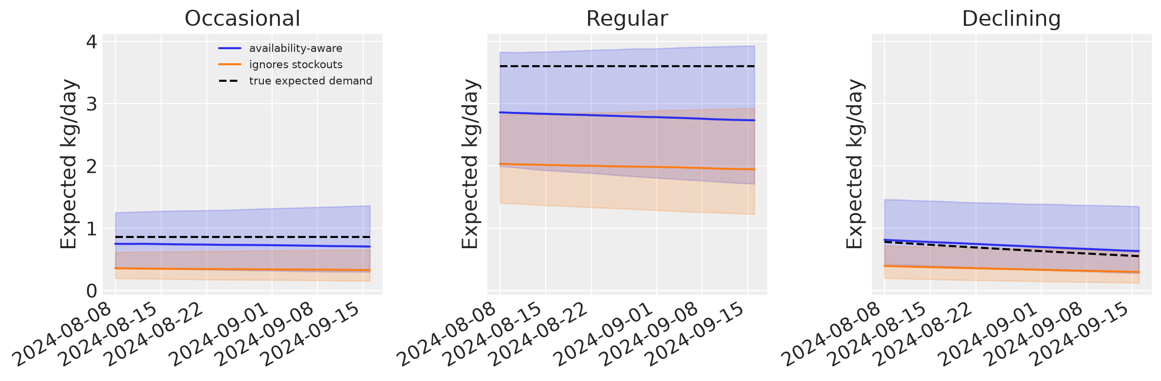
Refit the same model treating every historical zero as a possible non-occurrence. Comparing its full-availability forecast with the availability-aware fit shows how stockout zeros can bias estimated demand. In this simulation we know true demand; in real data assess demand forecasts on reliably available periods or against an independent demand measurement.

naive_inputs = train_inputs.copy(deep=True)
naive_inputs.loc[{"input": "available"}] = 1.0
naive_fc = HMCForecaster(
    demand_model,
    train,
    naive_inputs,
    draws=DRAWS,
    tune=TUNE,
    chains=CHAINS,
    random_seed=SEED + 4,
    progressbar=False,
    sample_kwargs={"target_accept": 0.9},
)
naive = naive_fc.forecast(
    future_covariates=full_inputs, num_samples=N_PRED, random_seed=SEED + 5
).predictions
rows = []
for product in products:
    for label, samples in [
        ("availability-aware", full.forecast),
        ("ignores stockouts", naive.forecast),
    ]:
        rows.append(
            {
                "product": product,
                "model": label,
                **evaluate_forecast(
                    samples.sel(product=product), truth_demand.sel(product=product)
                ),
            }
        )
pd.DataFrame(rows).set_index(["product", "model"]).round(3)

Initializing NUTS using jitter+adapt_diag...

Multiprocess sampling (2 chains in 2 jobs)

NUTS: [occurrence_intercept, occurrence_slope, positive_mean, positive_shape]

Sampling 2 chains for 800 tune and 600 draw iterations (1_600 + 1_200 draws total) took 1 seconds.

We recommend running at least 4 chains for robust computation of convergence diagnostics

The rhat statistic is larger than 1.01 for some parameters. This indicates problems during sampling. See https://arxiv.org/abs/1903.08008 for details

/Users/juanitorduz/.paseo/worktrees/1dtaxlkh/docs-example-notebook-visual-style/.venv/lib/python3.14/site-packages/pymc/distributions/mixture.py:311: MixtureTransformWarning: No safe default transform found for Mixture distribution forecast. This can happen when components have different supports or default transforms.
If appropriate, you can specify a custom transform for more efficient sampling.
  transform_warning()
Sampling: [forecast]

		mae	rmse	crps	coverage
product	model
Occasional	availability-aware	0.553	1.337	0.481	1.000
	ignores stockouts	0.553	1.342	0.492	0.900
Regular	availability-aware	1.743	3.290	1.453	0.975
	ignores stockouts	1.743	3.176	1.400	0.950
Declining	availability-aware	0.868	2.390	0.779	0.950
	ignores stockouts	0.868	2.432	0.804	0.900

The shaded bands below are 90% credible intervals for expected demand, excluding occurrence and quantity noise. Predictive intervals for actual daily demand would be much wider and include zeros.

fig, axes = plt.subplots(1, 3, figsize=(12, 4), sharey=True)
for ax, product in zip(axes, products, strict=True):
    for label, prediction, color in [
        ("availability-aware", full, "C0"),
        ("ignores stockouts", naive, "C1"),
    ]:
        mean = prediction.mu_future.sel(product=product)
        q = mean.quantile([0.05, 0.5, 0.95], dim=("chain", "draw"))
        ax.fill_between(
            time[n_train:], q.sel(quantile=0.05), q.sel(quantile=0.95), alpha=0.2, color=color
        )
        ax.plot(time[n_train:], q.sel(quantile=0.5), color=color, label=label)
    j = products.index(product)
    ax.plot(
        time[n_train:],
        probability[n_train:, j] * size_mean[j],
        color="black",
        ls="--",
        label="true expected demand",
    )
    ax.set(title=product, ylabel="Expected kg/day")
axes[0].legend(fontsize=8)
fig.autofmt_xdate()
fig.tight_layout()
plt.show()

/var/folders/cm/3dzy9rdd5s3672z0s1brjkvh0000gn/T/ipykernel_69767/3271208936.py:24: UserWarning: The figure layout has changed to tight
  fig.tight_layout()

Evaluate the business quantity you forecast

The table scores full-availability demand forecasts against simulated latent demand. A sales forecast should instead be scored against sales under the specified availability. These targets differ: low sales during stockouts do not establish that demand was low. Short, intermittent holdouts also make aggregate CRPS and coverage variable; inspect multiple origins and occurrence calibration before preferring a model.

The full-availability scenario estimates demand under the stated observation model. It does not establish a causal effect of stocking decisions. The model assumes known, external availability and does not cover noisy stockout labels or binding inventory caps. See the retail stockouts example for fractional availability.