Local level two ways: scan-based Markov latents vs. pymc-extras statespace#
The same generative model — a random-walk level observed with noise — can be written in
pymc_forecast in two ways:
Scan-based (
markov_series): the level is an explicit per-step latent sampled by NUTS, and the forecast segment is seeded from the final in-sample state.Statespace (
pymc_extras.statespaceviaStatespaceForecaster): the level is a linear-Gaussian hidden state that the Kalman filter marginalizes out exactly, so NUTS only samples the (few) structural parameters.
For linear-Gaussian dynamics the second form should win on both posterior quality
(no funnel between the level path and its innovation scale) and runtime (a handful of
parameters instead of one latent per time step). This notebook checks that claim on
simulated data with known parameters, and shows that both model kinds run through the same
backtest call and metrics.
Prepare notebook#
import logging
import os
from time import perf_counter

import arviz as az
import matplotlib.pyplot as plt
import numpy as np
import pandas as pd
import pymc as pm
import pytensor.tensor as pt
import xarray as xr
from pymc_extras.statespace import structural as st

from pymc_forecast import (
    HMCForecaster,
    Horizon,
    StatespaceForecaster,
    StatespaceModel,
    backtest,
    evaluate_forecast,
    markov_series,
    null_covariates,
    predict,
    results_to_dataframe,
)
from pymc_forecast.data import FUTURE_DIM, TIME_DIM

HDI_PROB = 0.94

az.style.use("arviz-darkgrid")
az.rcParams["stats.ci_kind"] = "hdi"
az.rcParams["stats.ci_prob"] = HDI_PROB
plt.rcParams["figure.figsize"] = [10, 6]
plt.rcParams["figure.dpi"] = 100
plt.rcParams["figure.facecolor"] = "white"

%config InlineBackend.figure_format = "retina"

logging.getLogger("pymc").setLevel(logging.ERROR)
logging.getLogger("pymc_extras").setLevel(logging.ERROR)

SEED = 20260713
rng = np.random.default_rng(SEED)

# CI executes every example notebook end-to-end with reduced settings.
SMOKE_TEST = os.environ.get("PYMC_FORECAST_SMOKE_TEST", "0") == "1"
DRAWS = 50 if SMOKE_TEST else 1_000
TUNE = 50 if SMOKE_TEST else 1_000
CHAINS = 2 if SMOKE_TEST else 4
NUM_SAMPLES = 50 if SMOKE_TEST else 1_000
BACKTEST_DRAWS = 50 if SMOKE_TEST else 500
BACKTEST_SAMPLES = 50 if SMOKE_TEST else 500
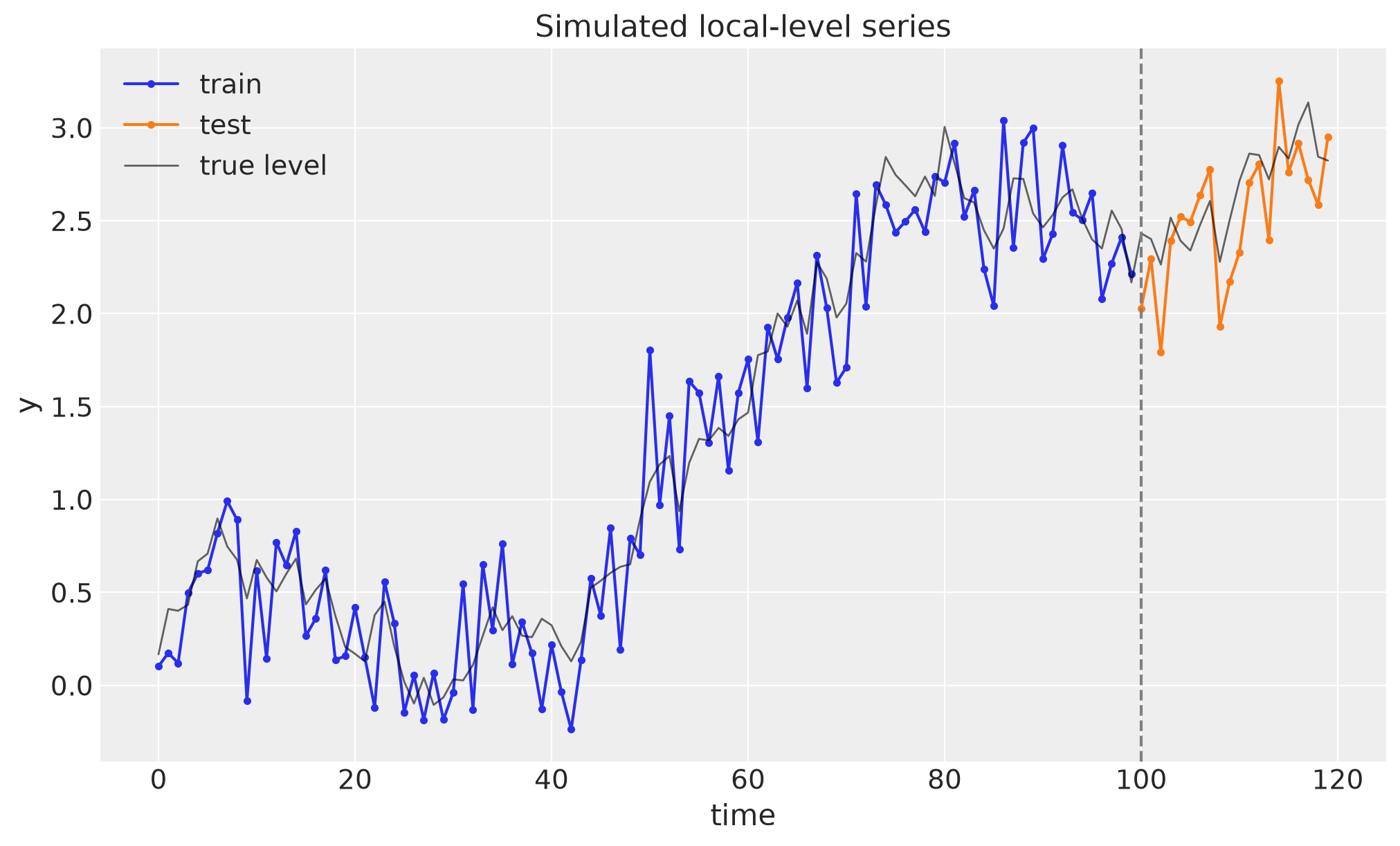
Simulate a local-level process#
A random-walk level with innovation scale \(\sigma_\eta = 0.15\), observed with noise \(\sigma_\varepsilon = 0.3\):
Knowing the true parameters lets us judge the posteriors, not just the forecasts.
SIGMA_LEVEL = 0.15
SIGMA_OBS = 0.3

n = 120
n_train = 100
future = n - n_train

level_true = np.cumsum(rng.normal(0.0, SIGMA_LEVEL, size=n))
y = level_true + rng.normal(0.0, SIGMA_OBS, size=n)

t = np.arange(n)
train_data = xr.DataArray(y[:n_train], dims=(TIME_DIM,), coords={TIME_DIM: t[:n_train]})
test_data = xr.DataArray(y[n_train:], dims=(TIME_DIM,), coords={TIME_DIM: t[n_train:]})
covariates_full = null_covariates(t)

fig, ax = plt.subplots()
ax.plot(t[:n_train], y[:n_train], "o-", color="C0", markersize=3, label="train")
ax.plot(t[n_train:], y[n_train:], "o-", color="C1", markersize=3, label="test")
ax.plot(t, level_true, color="black", linewidth=1, alpha=0.6, label="true level")
ax.axvline(n_train, color="gray", linestyle="--")
ax.legend(loc="upper left")
ax.set(title="Simulated local-level series", xlabel="time", ylabel="y")
plt.show()
Model 1: scan-based Markov latent#
markov_series samples the level path step by step with pytensor.scan; the
forecast segment is a second scan seeded from the final in-sample level. All 100
per-step latents are parameters of the NUTS run.
def scan_local_level(covariates, data=None) -> None:
    h = Horizon.from_data(covariates, data)
    sigma_level = pm.HalfNormal("sigma_level", 0.5)
    sigma_obs = pm.HalfNormal("sigma_obs", 0.5)
    level_init = pm.Normal("level_init", 0.0, 1.0)
    level = markov_series(
        h,
        "level",
        level_init,
        lambda z_prev, sigma: pm.Normal.dist(z_prev, sigma),
        params=(sigma_level,),
    )

    def obs_fn(name, mu, dims, observed):
        return pm.Normal(name, mu, sigma_obs, dims=dims, observed=observed)

    predict(h, obs_fn, level)


start = perf_counter()
scan_forecaster = HMCForecaster(
    scan_local_level,
    train_data,
    covariates_full,
    draws=DRAWS,
    tune=TUNE,
    chains=CHAINS,
    random_seed=SEED,
    sample_kwargs={"target_accept": 0.95},
)
scan_fit_seconds = perf_counter() - start
print(f"scan model fit: {scan_fit_seconds:.1f}s")
scan model fit: 5.8s
Model 2: statespace local level#
The same dynamics as a pymc_extras.statespace structural model:
LevelTrend(order=1, innovations_order=[1]) is exactly a random-walk level, plus
MeasurementError for \(\sigma_\varepsilon\). The Kalman filter integrates the level path
out analytically, so NUTS samples only the three structural parameters. The initial state
covariance P0 is fixed near zero so the initial state is effectively the sampled
initial_level_trend — the exact counterpart of the scan model’s level_init.
The StatespaceModel definition mirrors the statespace lifecycle: statespace() builds
the component graph, priors() declares the parameter priors (matched to the scan model’s
priors above).
class StatespaceLocalLevel(StatespaceModel):
    def statespace(self, data, covariates):
        level = st.LevelTrend(order=1, innovations_order=[1])
        return (level + st.MeasurementError()).build(verbose=False)

    def priors(self, ss_mod, data, covariates):
        # P0 ~ 0 pins the initial state to initial_level_trend ~ N(0, 1),
        # matching the scan model's level_init prior exactly
        pm.Deterministic("P0", 1e-4 * pt.eye(ss_mod.k_states), dims=("state", "state_aux"))
        pm.Normal("initial_level_trend", 0.0, 1.0, dims="state_level_trend")
        pm.HalfNormal("sigma_level_trend", 0.5, dims="shock_level_trend")
        pm.HalfNormal("sigma_MeasurementError", 0.5)


start = perf_counter()
ss_forecaster = StatespaceForecaster(
    StatespaceLocalLevel(),
    train_data,
    covariates_full,
    draws=DRAWS,
    tune=TUNE,
    chains=CHAINS,
    random_seed=SEED,
    sample_kwargs={"target_accept": 0.95},
)
ss_fit_seconds = perf_counter() - start
print(f"statespace model fit: {ss_fit_seconds:.1f}s")
statespace model fit: 4.4s
Posterior quality#
Both models estimate the same two scales. The table compares their posteriors against the truth, along with effective sample sizes and sampling efficiency (ESS per second — the number that actually matters when the two runs cost different amounts of wall clock).
scan_post = scan_forecaster.idata.posterior
ss_post = ss_forecaster.idata.posterior

pairs = [
    ("sigma_level", scan_post["sigma_level"], ss_post["sigma_level_trend"].squeeze(), SIGMA_LEVEL),
    ("sigma_obs", scan_post["sigma_obs"], ss_post["sigma_MeasurementError"], SIGMA_OBS),
]

rows = []
for name, scan_da, ss_da, truth in pairs:
    for model, da, seconds in [
        ("scan", scan_da, scan_fit_seconds),
        ("statespace", ss_da, ss_fit_seconds),
    ]:
        ess = float(np.asarray(az.ess(da.rename(name)).squeeze()))
        rows.append(
            {
                "parameter": name,
                "model": model,
                "truth": truth,
                "posterior mean": float(da.mean()),
                "posterior sd": float(da.std()),
                "ess_bulk": round(ess),
                "ess / second": round(ess / seconds, 1),
            }
        )

pd.DataFrame(rows).set_index(["parameter", "model"]).round(3)
| truth | posterior mean | posterior sd | ess_bulk | ess / second | ||
|---|---|---|---|---|---|---|
| parameter | model | |||||
| sigma_level | scan | 0.15 | 0.147 | 0.028 | 432 | 74.8 |
| statespace | 0.15 | 0.145 | 0.028 | 3338 | 751.5 | |
| sigma_obs | scan | 0.30 | 0.279 | 0.026 | 2766 | 478.5 |
| statespace | 0.30 | 0.280 | 0.026 | 3386 | 762.3 |
fig, axes = plt.subplots(1, 2, figsize=(12, 4))
for ax, (name, scan_da, ss_da, truth) in zip(axes, pairs, strict=True):
    bins = np.histogram_bin_edges(np.r_[scan_da.values.ravel(), ss_da.values.ravel()], bins=60)
    ax.hist(scan_da.values.ravel(), bins=bins, density=True, alpha=0.6, color="C0", label="scan")
    ax.hist(
        ss_da.values.ravel(), bins=bins, density=True, alpha=0.6, color="C2", label="statespace"
    )
    ax.axvline(truth, color="black", linestyle="--", label="truth")
    ax.set_title(name)
    ax.legend()
fig.suptitle("Innovation and observation scales: posterior vs truth")
plt.show()
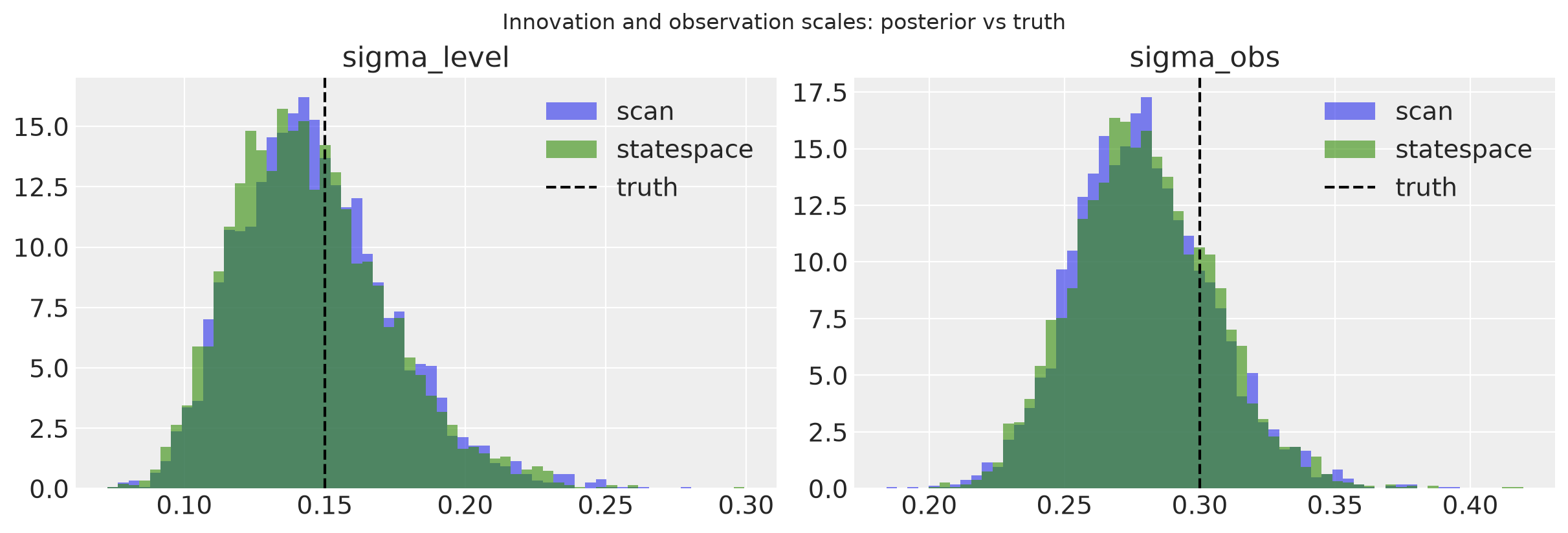
Both posteriors land on the truth, but the sampling efficiency differs sharply on the innovation scale \(\sigma_\eta\): sampling per-step latents couples the level path with its scale in a funnel-like geometry that NUTS has to fight through (low ESS despite 4000 draws), while the marginalized likelihood removes those latents entirely. At this series length the wall-clock per fit is compile-dominated and similar; the ESS-per-second gap is what grows as series get longer and models gain more per-step latents.
Forecasts#
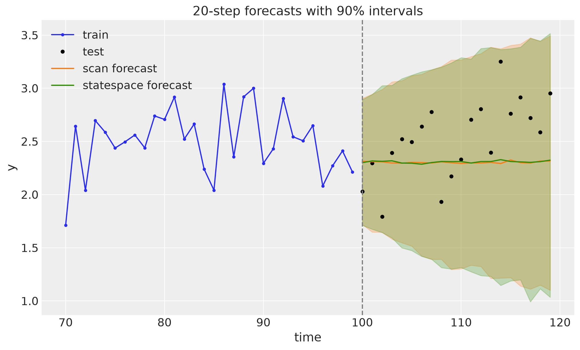
Both forecasters expose the same forecast API and return the same labeled
predictions group, so evaluation code does not care which one produced it.
num_samples = NUM_SAMPLES
scan_pred = scan_forecaster.forecast(covariates_full, num_samples=num_samples, random_seed=SEED)
ss_pred = ss_forecaster.forecast(covariates_full, num_samples=num_samples, random_seed=SEED)

scan_fc = scan_pred["predictions"]["forecast"]
ss_fc = ss_pred["predictions"]["forecast"]

scores = pd.DataFrame(
    {
        "scan": evaluate_forecast(scan_fc, test_data.rename({TIME_DIM: FUTURE_DIM})),
        "statespace": evaluate_forecast(ss_fc, test_data.rename({TIME_DIM: FUTURE_DIM})),
    }
)
scores.round(3)
| scan | statespace | |
|---|---|---|
| mae | 0.353 | 0.338 |
| rmse | 0.420 | 0.415 |
| crps | 0.241 | 0.236 |
| coverage | 1.000 | 1.000 |
fig, ax = plt.subplots()
ax.plot(t[70:n_train], y[70:n_train], "o-", color="C0", markersize=3, label="train")
ax.plot(t[n_train:], y[n_train:], "o", color="black", markersize=4, label="test")
for fc, color, label in [(scan_fc, "C1", "scan"), (ss_fc, "C2", "statespace")]:
    stacked = fc.stack(sample=("chain", "draw"))
    mean = stacked.mean("sample")
    lo, hi = stacked.quantile([0.05, 0.95], dim="sample").values
    ax.plot(fc[FUTURE_DIM].values, mean, color=color, label=f"{label} forecast")
    ax.fill_between(fc[FUTURE_DIM].values, lo, hi, color=color, alpha=0.25)
ax.axvline(n_train, color="gray", linestyle="--")
ax.legend(loc="upper left")
ax.set(title="20-step forecasts with 90% intervals", xlabel="time", ylabel="y")
plt.show()
One backtest call for both#
The point of the interop: backtest takes forecaster_cls= and per-window options, so a
statespace structural model is scored over the same moving windows, with the same metrics,
as a hand-written forecasting model. (Window schedules are reduced here to keep the
notebook quick.)
window_kwargs = dict(
    min_train_window=80,
    test_window=20,
    stride=20,
    num_samples=BACKTEST_SAMPLES,
    random_seed=SEED,
)

fit_options = {
    "draws": BACKTEST_DRAWS,
    "tune": BACKTEST_DRAWS,
    "chains": 2,
    "sample_kwargs": {"target_accept": 0.95},
}
scan_results = backtest(
    y,
    None,
    scan_local_level,
    forecaster_cls=HMCForecaster,
    forecaster_options=fit_options,
    **window_kwargs,
)
ss_results = backtest(
    y,
    None,
    StatespaceLocalLevel(),
    forecaster_cls=StatespaceForecaster,
    forecaster_options=fit_options,
    **window_kwargs,
)

comparison = pd.concat(
    {
        "scan": results_to_dataframe(scan_results).set_index("t1"),
        "statespace": results_to_dataframe(ss_results).set_index("t1"),
    },
    names=["model"],
)
columns = ["t0", "t2", "mae", "rmse", "crps", "coverage", "train_walltime", "test_walltime"]
comparison[columns].round(3)
The effective sample size per chain is smaller than 100 for some parameters. A higher number is needed for reliable rhat and ess computation. See https://arxiv.org/abs/1903.08008 for details
The effective sample size per chain is smaller than 100 for some parameters. A higher number is needed for reliable rhat and ess computation. See https://arxiv.org/abs/1903.08008 for details
| t0 | t2 | mae | rmse | crps | coverage | train_walltime | test_walltime | ||
|---|---|---|---|---|---|---|---|---|---|
| model | t1 | ||||||||
| scan | 80 | 0 | 100 | 0.259 | 0.303 | 0.200 | 1.0 | 1.786 | 0.122 |
| 100 | 0 | 120 | 0.350 | 0.425 | 0.241 | 1.0 | 2.195 | 0.075 | |
| statespace | 80 | 0 | 100 | 0.264 | 0.311 | 0.204 | 1.0 | 2.773 | 0.488 |
| 100 | 0 | 120 | 0.377 | 0.449 | 0.254 | 1.0 | 2.909 | 0.707 |
Takeaways#
Same protocol:
StatespaceForecastersatisfies the forecaster interface, so statespace models drop intoforecast,predict_in_sample,backtest, and the metrics layer unchanged.Better sampling for linear-Gaussian dynamics: Kalman-filter marginalization removes the per-step latents from the sampling problem — several-fold more effective samples per second on the innovation scale (~7x the bulk ESS in this run), with forecasts and calibration on par. (On a 100-step series the total wall clock is compile-dominated and similar; the efficiency gap is what scales.)
When to scan:
markov_seriesremains the tool for nonlinear or non-Gaussian transitions (thresholds, multiplicative dynamics, discrete or heavy-tailed innovations) that a linear-Gaussian statespace cannot express.